程式師世界 >> 編程語言 >> C語言 >> C++ >> C++入門知識 >> Interpolation methods，interpolation

Interpolation methods，interpolation

編輯：C++入門知識

Interpolation methods，interpolation

Written by Paul Bourke
December 1999

Discussed here are a number of interpolation methods, this is by no means an exhaustive list but the methods shown tend to be those in common use in computer graphics. The main attributes is that they are easy to compute and are stable. Interpolation as used here is different to "smoothing", the techniques discussed here have the characteristic that the estimated curve passes through all the given points. The idea is that the points are in some sense correct and lie on an underlying but unknown curve, the problem is to be able to estimate the values of the curve at any position between the known points.

Linear interpolation is the simplest method of getting values at positions in between the data points. The points are simply joined by straight line segments. Each segment (bounded by two data points) can be interpolated independently. The parameter mu defines where to estimate the value on the interpolated line, it is 0 at the first point and 1 and the second point. For interpolated values between the two points mu ranges between 0 and 1. Values of mu outside this range result in extrapolation. This convention is followed for all the subsequent methods below. As with subsequent more interesting methods, a snippet of plain C code will server to describe the mathematics.

double LinearInterpolate(
   double y1,double y2,
   double mu)
{
   return(y1*(1-mu)+y2*mu);
}

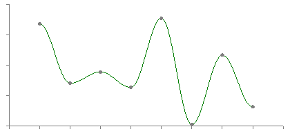
Linear interpolation results in discontinuities at each point. Often a smoother interpolating function is desirable, perhaps the simplest is cosine interpolation. A suitable orientated piece of a cosine function serves to provide a smooth transition between adjacent segments.

double CosineInterpolate(
   double y1,double y2,
   double mu)
{
   double mu2;

   mu2 = (1-cos(mu*PI))/2;
   return(y1*(1-mu2)+y2*mu2);
}

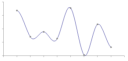
Cubic interpolation is the simplest method that offers true continuity between the segments. As such it requires more than just the two endpoints of the segment but also the two points on either side of them. So the function requires 4 points in all labeled y0, y1, y2, and y3, in the code below. mu still behaves the same way for interpolating between the segment y1 to y2. This does raise issues for how to interpolate between the first and last segments. In the examples here I just haven't bothered. A common solution is the dream up two extra points at the start and end of the sequence, the new points are created so that they have a slope equal to the slope of the start or end segment.

double CubicInterpolate(
   double y0,double y1,
   double y2,double y3,
   double mu)
{
   double a0,a1,a2,a3,mu2;

   mu2 = mu*mu;
   a0 = y3 - y2 - y0 + y1;
   a1 = y0 - y1 - a0;
   a2 = y2 - y0;
   a3 = y1;

   return(a0*mu*mu2+a1*mu2+a2*mu+a3);
}

Paul Breeuwsma proposes the following coefficients for a smoother interpolated curve, which uses the slope between the previous point and the next as the derivative at the current point. This results in what are generally referred to as Catmull-Rom splines.

   a0 = -0.5*y0 + 1.5*y1 - 1.5*y2 + 0.5*y3;
   a1 = y0 - 2.5*y1 + 2*y2 - 0.5*y3;
   a2 = -0.5*y0 + 0.5*y2;
   a3 = y1;

Hermite interpolation like cubic requires 4 points so that it can achieve a higher degree of continuity. In addition it has nice tension and biasing controls. Tension can be used to tighten up the curvature at the known points. The bias is used to twist the curve about the known points. The examples shown here have the default tension and bias values of 0, it will be left as an exercise for the reader to explore different tension and bias values.

/*
   Tension: 1 is high, 0 normal, -1 is low
   Bias: 0 is even,
         positive is towards first segment,
         negative towards the other
*/
double HermiteInterpolate(
   double y0,double y1,
   double y2,double y3,
   double mu,
   double tension,
   double bias)
{
   double m0,m1,mu2,mu3;
   double a0,a1,a2,a3;

	mu2 = mu * mu;
	mu3 = mu2 * mu;
   m0  = (y1-y0)*(1+bias)*(1-tension)/2;
   m0 += (y2-y1)*(1-bias)*(1-tension)/2;
   m1  = (y2-y1)*(1+bias)*(1-tension)/2;
   m1 += (y3-y2)*(1-bias)*(1-tension)/2;
   a0 =  2*mu3 - 3*mu2 + 1;
   a1 =    mu3 - 2*mu2 + mu;
   a2 =    mu3 -   mu2;
   a3 = -2*mu3 + 3*mu2;

   return(a0*y1+a1*m0+a2*m1+a3*y2);
}

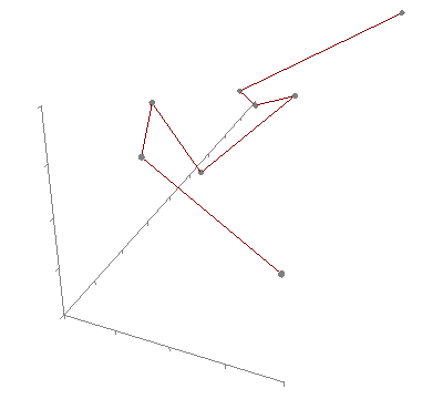
While you may think the above cases were 2 dimensional, they are just 1 dimensional interpolation (the horizontal axis is linear). In most cases the interpolation can be extended into higher dimensions simply by applying it to each of the x,y,z coordinates independently. This is shown on the right for 3 dimensions for all but the cosine interpolation. By a cute trick the cosine interpolation reverts to linear if applied independently to each coordinate.

For other interpolation methods see the Bezier, Spline, and piecewise Bezier methods here.

Linear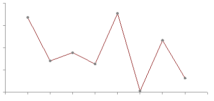

Cosine

Cubic

Hermite

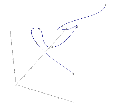
3D linear

3D cubic

3D Hermite

Trilinear Interpolation

Written by Paul Bourke
July 1997

Trilinear interpolation is the name given to the process of linearly interpolating points within a box (3D) given values at the vertices of the box. Perhaps its most common application is interpolating within cells of a volumetric dataset.

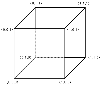
Consider a unit cube with the lower/left/base vertex at the origin as shown here on the right.
The values at each vertex will be denoted V₀₀₀, V₁₀₀, V₀₁₀, ....etc....V₁₁₁

The value at position (x,y,z) within the cube will be denoted V_xyz and is given by

V_xyz = V₀₀₀ (1 - x) (1 - y) (1 - z) +
V₁₀₀ x (1 - y) (1 - z) +
V₀₁₀ (1 - x) y (1 - z) +
V₀₀₁ (1 - x) (1 - y) z +
V₁₀₁ x (1 - y) z +
V₀₁₁ (1 - x) y z +
V₁₁₀ x y (1 - z) +
V₁₁₁ x y z

In general the box will not be of unit size nor will it be aligned at the origin. Simple translation and scaling (possibly of each axis independently) can be used to transform into and then out of this simplified situation.

Linear Regression

Written by Paul Bourke
October 1998

Linear regression is a method to best fit a linear equation (straight line) of the form y(x) = a + b x to a collection of N points (x_i,y_i). Where b is the slope and a the intercept on the y axis.

The result will be stated below without derivation, that requires minimisation of the sum of the squared distance from the data points and the proposed line. This function is minimised by calculating the derivative with respect to a and b and setting these to zero. For a more complete derivation see the "Numerical Recipes in C".

The solution is clearer if we define the following

Then

and

And finally the regression coefficient is

This is 0 if there is no linear trend, 1 for perfect linear fit.

Note

This discussion assumes there is no known variance for the x and y values. There are solutions which can take this into account, this is particularly important if some values are known with less error than others.
The solution above requires that the slope is not infinite, S_xx is not zero.

Example

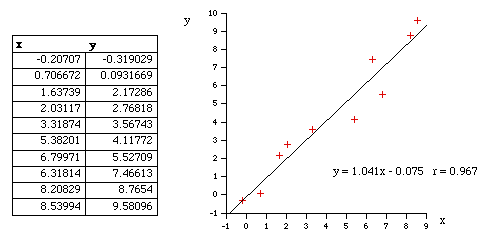
The following example shows the points and the best fit line as determined using the techniques discussed here.

Source

C
linregress.c

C++ contributed by Charles Brown
RegressionLine.cpp
RegressionLine.hpp

Curve Fit Through Arbitrary Points

Written by Paul Bourke
August 1991

The following introduces a method of immediately deriving a polynomial that passes through an arbitrary number of points. That is, find a polynomial f(x) that passes through the N points

(x₀,y₀), (x₁,y₁), (x₂,y₂), ..... (x_N-1,y_N-1)

The key to this solution is that we want an exact fit at the points given and we don't care what happens in between those points. The general solution is

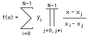
To see how this works, consider the product term. When x = x_i the product term has the same denominator and numerator and thus equals 1 and therefore contributes y_i to the sum. All other terms in the summation contribute 0 since there exists a (x_j - x_j) in the numerator. Thanks to Simon Stegmaier for pointing out that this is known as a Lagrange Polynomial.

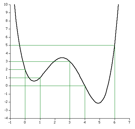
For a numerical example consider the polynomial that passes through the following points

(0,2)
(1,1)
(3,3)
(4,0)
(6,5)

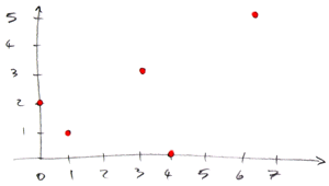
The function using the above formula is

   f(x) = 2 * (x-1) * (x-3) * (x-4) * (x-6) / [ (0-1) * (0-3) * (0-4) * (0-6) ]
        + 1 * (x-0) * (x-3) * (x-4) * (x-6) / [ (1-0) * (1-3) * (1-4) * (1-6) ]
        + 3 * (x-0) * (x-1) * (x-4) * (x-6) / [ (3-0) * (3-1) * (3-4) * (3-6) ]
        + 0 * (x-0) * (x-1) * (x-3) * (x-6) / [ (4-0) * (4-1) * (4-3) * (4-6) ]
        + 5 * (x-0) * (x-1) * (x-3) * (x-4) / [ (6-0) * (6-1) * (6-3) * (6-4) ]

   f(x) = (x-1) * (x-3) * (x-4) * (x-6) / 36
        - (x-0) * (x-3) * (x-4) * (x-6) / 30
        + (x-0) * (x-1) * (x-4) * (x-6) / 6 
        + (x-0) * (x-1) * (x-3) * (x-4) / 36

   f(x) = 17*x

⁴

/90 - 181*x

/90 + 563*x

/90 - 163*x/30 + 2

By substituting the values of x for the points the function must pass through (x=0,1,3,4,6) it is easy to see that the expression above achieves the result, namely y=2,1,3,0,5 respectively.

What happens at other points?

All bets are off regarding the behavior between the fixed points. The polynomial is of degree N and could violently fly off anywhere. The continuous curve for the numerical example above is shown below.

A competition in the Mathematics news groups in October 1998

From: "John Santos" <[email protected]>
Newsgroups: alt.sci.math.probability,alt.tv.mathnet,aus.mathematics
Subject: $100.00 prize for the solution
Date: Tue, 15 Sep 1998 20:56:50 -0700
X-Newsreader: Microsoft Outlook Express 4.72.3110.1
X-MimeOLE: Produced By Microsoft MimeOLE V4.72.3110.3
NNTP-Posting-Host: 209.239.197.111
X-NNTP-Posting-Host: 209.239.197.111
Message-ID: <[email protected]>
X-NNTP-Posting-Host: 209.63.114.134

Hi everyone,
My name is John Santos and I am willing to pay anyone $100.00 for the first
person to solve this problem. I am providing some hints. This works as follows:
you will see nine digits - the tenth digit or letter is the answer. 
What I need is the formula or mathematical equation to get there...

   Number          Answer 
---------------------------
   749736637         1     
   713491024         8     
   523342792         D     
   749236871         P     
   727310078         E     
   746261832         4     
   733237527         L     
   743510589         9     
   715240338         K     
   722592910         1     
   739627071         R     

The first one with the answer and emails it to me wins the $100.00
Email address: [email protected]
Good Luck !!!!

They refused to pay up for this solution !!!!

My reply to this posting was

The following is the solution to the posted problem, although it probably 
doesn't offer the insight you are seeking, it certainly falls within the 
scope of competition. To illustrate my solution I will use the following 
symbols instead of the numbers you used simply to save space. For your 
second column with letters and numbers use their ASCII values instead, 
this has no loss of generality as it is a simple 1 to 1 mapping.

x1 y1
x2 y2
x3 y3
x4 y4
etc

The following is a general method of making a function that passes 
through any pair of values (xi,yi).

        y1 (x-x2) (x-x3) (x-x4)
f(x) = --------------------------- 
         (x1-x2) (x1-x3) (x1-x4)

        y2 (x-x1) (x-x3) (x-x4)
     + --------------------------- 
         (x2-x1) (x2-x3) (x2-x4)

        y3 (x-x1) (x-x2) (x-x4)
     + --------------------------- 
         (x3-x1) (x3-x2) (x3-x4)

        y4 (x-x1) (x-x2) (x-x3)
     + --------------------------- 
         (x4-x1) (x4-x2) (x4-x3)

etc etc. As you can see, at x=x1 all the terms disappear except the 
first which equals y1, at x=x2 all the terms disappear except the
second which equals y2, etc etc.

   X                           Y
   Number           Answer     ASCII
---------------------------------------
   749736637        1          49
   713491024        8          56
   523342792        D          68
   749236871        P          80
   727310078        E          69
   746261832        4          52
   733237527        L          76
   743510589        9          57
   715240338        K          75
   722592910        1          49
   739627071        R          82

The "lovely" expression in this case is
f(x) = + 49 ((x - 713491024) / 36245613) ((x - 523342792) / 226393845) ((x - 749236871) / 499766) ((x - 727310078) / 22426559) ((x - 746261832) / 3474805) ((x - 733237527) / 16499110) ((x - 743510589) / 6226048) ((x - 715240338) / 34496299) ((x - 722592910) / 27143727) ((x - 739627071) / 10109566) + 56 ((x - 749736637) / -36245613) ((x - 523342792) / 190148232) ((x - 749236871) / -35745847) ((x - 727310078) / -13819054) ((x - 746261832) / -32770808) ((x - 733237527) / -19746503) ((x - 743510589) / -30019565) ((x - 715240338) / -1749314) ((x - 722592910) / -9101886) ((x - 739627071) / -26136047) + 68 ((x - 749736637) / -226393845) ((x - 713491024) / -190148232) ((x - 749236871) / -225894079) ((x - 727310078) / -203967286) ((x - 746261832) / -222919040) ((x - 733237527) / -209894735) ((x - 743510589) / -220167797) ((x - 715240338) / -191897546) ((x - 722592910) / -199250118) ((x - 739627071) / -216284279) + 80 ((x - 749736637) / -499766) ((x - 713491024) / 35745847) ((x - 523342792) / 225894079) ((x - 727310078) / 21926793) ((x - 746261832) / 2975039) ((x - 733237527) / 15999344) ((x - 743510589) / 5726282) ((x - 715240338) / 33996533) ((x - 722592910) / 26643961) ((x - 739627071) / 9609800) + 69 ((x - 749736637) / -22426559) ((x - 713491024) / 13819054) ((x - 523342792) / 203967286) ((x - 749236871) / -21926793) ((x - 746261832) / -18951754) ((x - 733237527) / -5927449) ((x - 743510589) / -16200511) ((x - 715240338) / 12069740) ((x - 722592910) / 4717168) ((x - 739627071) / -12316993) + 52 ((x - 749736637) / -3474805) ((x - 713491024) / 32770808) ((x - 523342792) / 222919040) ((x - 749236871) / -2975039) ((x - 727310078) / 18951754) ((x - 733237527) / 13024305) ((x - 743510589) / 2751243) ((x - 715240338) / 31021494) ((x - 722592910) / 23668922) ((x - 739627071) / 6634761) + 76 ((x - 749736637) / -16499110) ((x - 713491024) / 19746503) ((x - 523342792) / 209894735) ((x - 749236871) / -15999344) ((x - 727310078) / 5927449) ((x - 746261832) / -13024305) ((x - 743510589) / -10273062) ((x - 715240338) / 17997189) ((x - 722592910) / 10644617) ((x - 739627071) / -6389544) + 57 ((x - 749736637) / -6226048) ((x - 713491024) / 30019565) ((x - 523342792) / 220167797) ((x - 749236871) / -5726282) ((x - 727310078) / 16200511) ((x - 746261832) / -2751243) ((x - 733237527) / 10273062) ((x - 715240338) / 28270251) ((x - 722592910) / 20917679) ((x - 739627071) / 3883518) + 75 ((x - 749736637) / -34496299) ((x - 713491024) / 1749314) ((x - 523342792) / 191897546) ((x - 749236871) / -33996533) ((x - 727310078) / -12069740) ((x - 746261832) / -31021494) ((x - 733237527) / -17997189) ((x - 743510589) / -28270251) ((x - 722592910) / -7352572) ((x - 739627071) / -24386733) + 49 ((x - 749736637) / -27143727) ((x - 713491024) / 9101886) ((x - 523342792) / 199250118) ((x - 749236871) / -26643961) ((x - 727310078) / -4717168) ((x - 746261832) / -23668922) ((x - 733237527) / -10644617) ((x - 743510589) / -20917679) ((x - 715240338) / 7352572) ((x - 739627071) / -17034161) + 82 ((x - 749736637) / -10109566) ((x - 713491024) / 26136047) ((x - 523342792) / 216284279) ((x - 749236871) / -9609800) ((x - 727310078) / 12316993) ((x - 746261832) / -6634761) ((x - 733237527) / 6389544) ((x - 743510589) / -3883518) ((x - 715240338) / 24386733) ((x - 722592910) / 17034161) f( 749736637) = 49 (1) f( 713491024) = 56 (8) f( 523342792) = 68 (D) f( 749236871) = 80 (P) f( 727310078) = 69 (E) f( 746261832) = 52 (4) f( 733237527) = 76 (L) f( 743510589) = 57 (9) f( 715240338) = 75 (K) f( 722592910) = 49 (1) f( 739627071) = 82 (R)