This article USES the python The language completes the data analysis and visualization of the cross-border transaction data set of online e-retail companies 、 According to the principle of association rules, the design and Implementation Based on Apriori The association rule mining program of the algorithm and encapsulate the program 、 Use the encapsulated association rule mining program to mine association rules on data sets , And analyze the mining results .
Dataset address :Online Retail | Kaggle https://www.kaggle.com/puneetbhaya/online-retail
Catalog
One 、 Algorithm principle
1.1 Association rules
1.2 Apriori Principle generates frequent itemsets
Two 、 Data preprocessing
2.1 Data description
2.2 Import the required third-party libraries 、 Reading data sets 、 View basic data set information
2.3 Data De duplication
2.4 Data outlier handling
2.5 Data missing value processing
3、 ... and 、 Statistics of sales volume in different countries
Four 、 Overall association rules
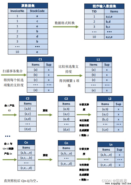
4.1. Execution principle of association rule program , The data is demonstration data , Is not Online Retail Data in data set .
4.2 Write data set format modification function , Generate suitable for Apriori Data format executed by algorithm program .
4.3 Write and generate association rule classes ( Encapsulate the association rule generator in a class , Convenient to call )
4.4 call Apriori class
5、 ... and 、 The main 3 Association rule analysis of countries
Association rules represent the correlation between items in the form of rules , The purpose is to find the relationship between items in a data set ( This relationship is often not directly reflected in the data ). And the discovered connections are expressed in the form of association rules or frequent itemsets .
Related concepts are explained as follows :
① Of association rules Support ( Relative support ):
Itemsets A、B The probability of simultaneous occurrence is called the support of association rules ( Relative support ).
Support ( A = > B ) = P ( A∪B )
② Of association rules Degree of confidence :
In itemset A Under the condition of occurrence , Then the itemset B The probability of occurrence is the confidence of association rules .
Confidence(A=>B)=P(B|A)
③ Of association rules Promotion :
finger A Xiang He B The frequency of items appearing together , But at the same time, consider the frequency of these two items .
{A→B} Lifting degree of ={A→B} The degree of confidence /P(B)=P(B|A)/P(B)= P(A∩B)/(P(A)*P(B)).
④ Minimum support : A threshold to measure support , Indicates the lowest statistical importance of the itemset .
⑤ Minimum confidence : A threshold to measure confidence , Represents the lowest reliability of association rules .
⑥ Strong rules : A rule that satisfies both the minimum support threshold and the minimum confidence threshold .
⑦ Itemsets : Collection of items . contain k The set of items is called k Itemsets , Such as assembly { milk , Oatmeal , sugar } It's a trinomial set . The frequency of itemsets is the count of all transactions that contain itemsets , Also known as absolute support or support count . If the itemset L The relative support of meets the predefined minimum support threshold , be L It's a frequent itemset . If there is K term , Write it down as Lk.
Apriori Algorithm is commonly used to mine data association rules , Be able to find data sets that frequently appear in the database , The rules formed by these connections can help users find some behavioral characteristics , In order to make enterprise decisions . for example , A food store hopes to discover customers' buying behavior , According to the analysis of shopping basket, most customers will buy bread and milk at the same time , Then the store can increase the sales of bread and milk while reducing prices to promote bread .
(1) Find all frequent itemsets ( Support is greater than or equal to the given support threshold )
① Connect
The purpose of the connection step is to find K Itemsets . For a given minimum support threshold , Respectively for 1 Item candidate set C1, Eliminate the item set whose support is less than the threshold, and get 1 Frequent item sets L1; The next step is L1 Self connection produces 2 Item candidate set C2, Eliminate the item set whose support is less than the threshold, and get 2 Frequent item sets L2; The next step is L2 and L1 Connection produces 3 Item candidate itemset C3; Eliminate the item set whose support is less than the threshold, and get 3 Frequent item sets L3; And it goes on , Until L(k-1) and L1 Connection produces k Item candidate set Ck, The maximum frequent itemset is obtained by eliminating itemsets smaller than the threshold Lk.
② prune
Pruning is followed by connecting steps , Generating candidate item sets Ck It plays the purpose of reducing the search space . according to Apriori The nature of , All non empty subsets of frequent itemsets must also be frequent itemsets , Therefore, the item set that does not meet this property will not exist in the candidate set C in , The process is pruning .
(2) Generate strong association rules from frequent itemsets
from (1) You know , Itemsets whose support does not exceed the support threshold have been rejected , If the remaining itemsets meet the predetermined confidence threshold , Then we can mine strong association rules , And calculate the promotion degree of the rule .
Apriori The detailed process and schematic diagram of the algorithm will be given in the operation section below .
The data set comes from an online e-retail company registered in the UK , stay 2010 year 12 month 1 The day is coming 2011 year 12 month 9 Online transaction data between dates , share 541909 Bar record 、8 A field .
The meaning of the field is as follows :
import matplotlib.pyplot as plt
import pandas as pd
import missingno as msno
import seaborn as sns
from matplotlib import cm
plt.rcParams['font.sans-serif'] = ['SimHei'] # Show Chinese tags
plt.rcParams['axes.unicode_minus'] = False
# Reading data
dataset = pd.read_excel("Online Retail.xlsx")
# View dataset dimensions
print(dataset.shape) # (541909, 8)
# View the data format of each column in the dataset
print(dataset.dtypes)
# Check the data distribution of each column
print(dataset.info())
print(dataset.describe())
The operation results are as follows :
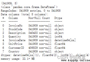
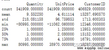
It can be seen that the data total 541909 strip , among “Description”、“CustomerID” There is missing data in two fields .“Quantity”、“UnitPrice” The minimum value of the field is negative , A negative number of product sales may be due to the return of goods , But this situation has a reverse effect on the generation of association rules ( Weaken the strength of Correlation ), Negative product sales unit price indicates abnormal data in this field .
Delete identical records .
dataset.drop_duplicates(inplace=True)
print(" Basic information of data after weight removal :")
# View dataset dimensions
print(dataset.shape) # (536641, 8)
# View the data format of each column in the dataset
print(dataset.dtypes)
# Check the data distribution of each column
print(dataset.info())
print(dataset.describe())
The operation results are as follows :

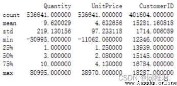
You can see , There are... In the dataset 5268 Completely repeated records , After deleting duplicate records , The data set is left 536641 Bar record .
Remove “Quantity”<= 0 or “UnitPrice”< 0 Abnormal records that do not conform to the actual situation .
print(" Data outlier handling :")
dataset = dataset.loc[(dataset["Quantity"]>0) & (dataset["UnitPrice"]>=0)]
print(dataset.describe())
The operation results are as follows :
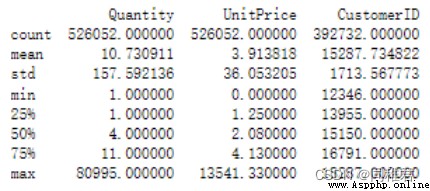
You can see , After removing the outliers, there are still 526052 Bar record .
Check for missing data
msno.matrix(dataset, labels=True, fontsize=9) # Matrix diagram
plt.show()
print(dataset.info())
The operation results are as follows :
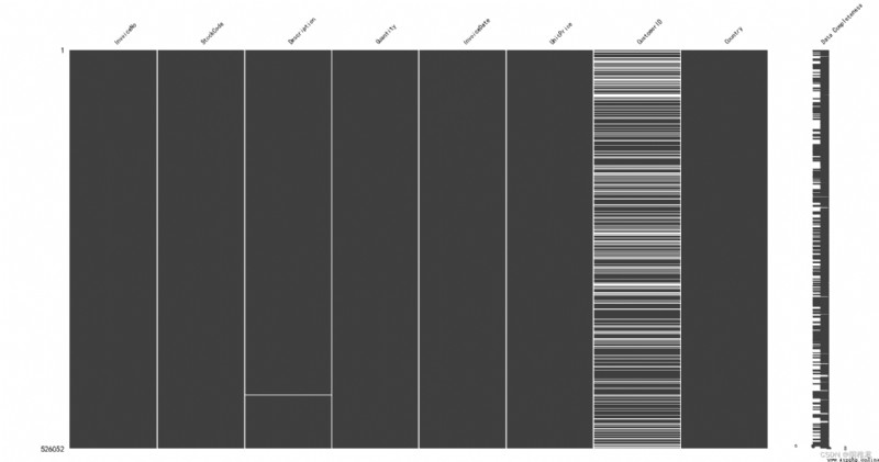
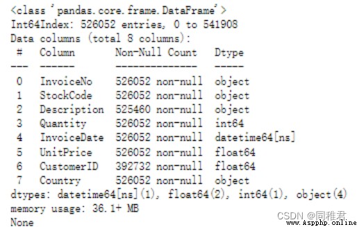
You can see “CustomerID” There are a lot of obvious deficiencies in field data ,“Description” There is a small amount of missing data in the field data . in consideration of “CustomerID” There is a great amount of missing field data , And the customer number is difficult to estimate , So delete in “CustomerID” There are records with missing values in the field .“Description” Describe for product information , Its missing amount is less , The description of the same product is the same , So it can be easily filled “Description” Empty value of field . because “Description” Fields have little effect on building association rules , So you can take it out separately later “StockCode” and “Description” Field , And remove the weight , Generate {“StockCode” : “Description”} Dictionaries , Used to find the corresponding product description according to the product number .
Delete on “CustomerID” There are records with missing values in the field
dataset["InvoiceNo"] = dataset["InvoiceNo"].astype("int")
print(dataset.info())
The operation results are as follows :
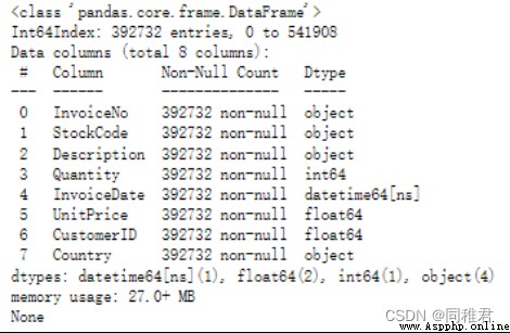
You can see , After removing the missing values , The dataset is left 392732 Bar record .
# According to the data set "Country" Field values are grouped
groupByCountry = dataset.groupby("Country")
# Of the data in each group "Quantity" Field to sum
country_quantity_list = list(dict(groupByCountry["Quantity"].sum()).items())
# Sort the data set according to the total product sales
country_quantity_list.sort(key=lambda x: x[1])
print("country_quantity_list:")
print(country_quantity_list)
The statistics are as follows :

Visualize the statistical results
# country_quantity_list.pop() # Remove during visualization / Keep the sales data of the country with the largest sales volume
norm = plt.Normalize(0, country_quantity_list[-1][1])
norm_values = norm([i[1] for i in country_quantity_list])
map_vir = cm.get_cmap(name='jet')
colors = map_vir(norm_values)
plt.barh([i[0] for i in country_quantity_list], [i[1] for i in country_quantity_list], height = 0.4,color=colors)
plt.tick_params(labelsize=8) # Set coordinate font size
sm = cm.ScalarMappable(cmap=map_vir, norm=norm) # norm Set max min
sm.set_array([])
plt.colorbar(sm)
# Add data labels to the bar chart
for index, y_value in enumerate([i[1] for i in country_quantity_list]):
plt.text(y_value+10, index-0.2, "%s" %y_value)
plt.ylabel("Country", fontdict={'size':18})
plt.title(" Total sales of products in different countries ")
plt.show() 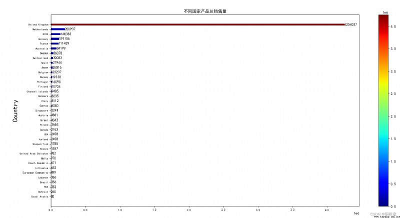
You can see the products of the store in United Kingdom The highest sales volume in , Far more than the total sales in the remaining countries . The top five countries in terms of sales volume are United Kingdom、Netherlands、EIRE、Germany、France.
In order to see the products more intuitively United Kingdom Sales in countries other than , Then draw no United Kingdom Bar chart of product sales .
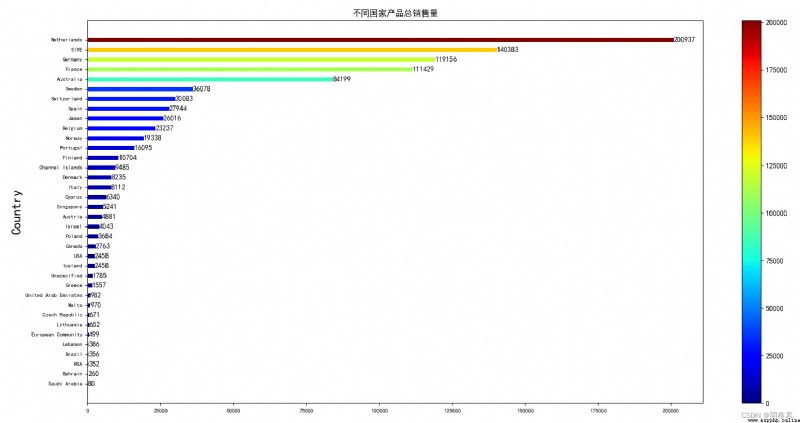
It can be seen that the export countries of the products of the store are mainly countries around the UK ( Like the Netherlands 、 The Irish ) And some of the most populous countries in Europe ( Such as Germany 、 The French ).
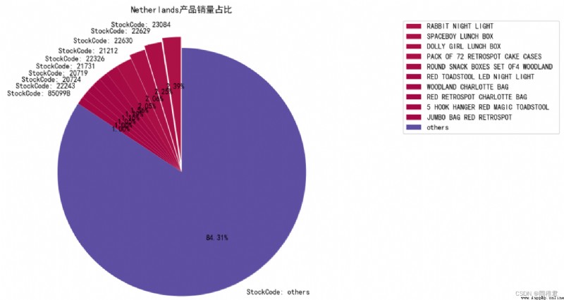
Separate statistics United Kingdom And Bahrain Sales of products in the country , And draw a pie chart of the top ten products in sales ( among others It means the first one 11 The total sales volume of the products ranking first to last ), The statistics of product sales ranking can reflect the correlation between some products to a certain extent , If the sales volume of the products ranking first is close to that of the products ranking second , Then there may be a strong correlation between these two products .
# Get the product code and its corresponding description
Sto_Des = dataset.loc[:,["StockCode","Description"]]
Sto_Des.dropna(inplace=True) # First remove the line with the missing product description
Sto_Des.drop_duplicates(inplace=True) # duplicate removal , Leave the only product StockCode And Description
# print("Sto_Des shape:",Sto_Des.shape)
# print("Sto_Des:", Sto_Des)
# Check the sales volume of each product in the top three countries
country_quantity_list.sort(key=lambda x: x[1], reverse=True)
for element in country_quantity_list[0:3]:
contryName = element[0]
# Get the grouping data of the corresponding country
df = groupByCountry.get_group(contryName)
# According to the product code StockCode Grouping
groupByStockCode = df.groupby("StockCode")
# Sum the total sales of a product respectively
country_StockCode_quantity_list = list(dict(groupByStockCode["Quantity"].sum()).items())
country_StockCode_quantity_list.sort(key=lambda x: x[1], reverse=True)
# After sales 10 Sum the sales volume of famous products , And named it "others"
othersQuantity = sum(list(i[1] for i in country_StockCode_quantity_list[10:]))
new_country_StockCode_quantity_list = country_StockCode_quantity_list[0:10] + [("others", othersQuantity)]
# Add corresponding description information for the product
# print(new_country_StockCode_quantity_list)
for i in range(len(new_country_StockCode_quantity_list)-1):
item = new_country_StockCode_quantity_list[i]
stockCode = item[0]
quantity = item[1]
description = Sto_Des["Description"].loc[Sto_Des["StockCode"]==item[0]]
new_country_StockCode_quantity_list[i] = (stockCode, quantity, list(description)[0])
# print(new_country_StockCode_quantity_list)
norm = plt.Normalize(0, max(new_country_StockCode_quantity_list, key=lambda x:x[1])[1])
# print(max(new_country_StockCode_quantity_list, key=lambda x:x[1])[1])
norm_values = norm([i[1] for i in new_country_StockCode_quantity_list])
map_vir = cm.get_cmap(name='Spectral')
# Produce continuous color matching
colors = map_vir(norm_values)
explode = [0.09, 0.06, 0.03] + [0]*(len(new_country_StockCode_quantity_list)-3)
plt.pie([i[1] for i in new_country_StockCode_quantity_list],
autopct='%.2f%%',
labels=["StockCode: " + str(i[0]) for i in new_country_StockCode_quantity_list],
explode=explode,
startangle=90,
colors=colors)
labels = [i[2] for i in new_country_StockCode_quantity_list[0:-1]] + ["others"]
plt.legend(labels,
loc="upper left",
bbox_to_anchor=(1.2, 0, 0.5, 1))
plt.title(f"{contryName} Proportion of product sales ")
plt.show()
The operation results are as follows :
United Kingdom
The list of products with the top ten sales volume is as follows :

The pie chart drawn is as follows :
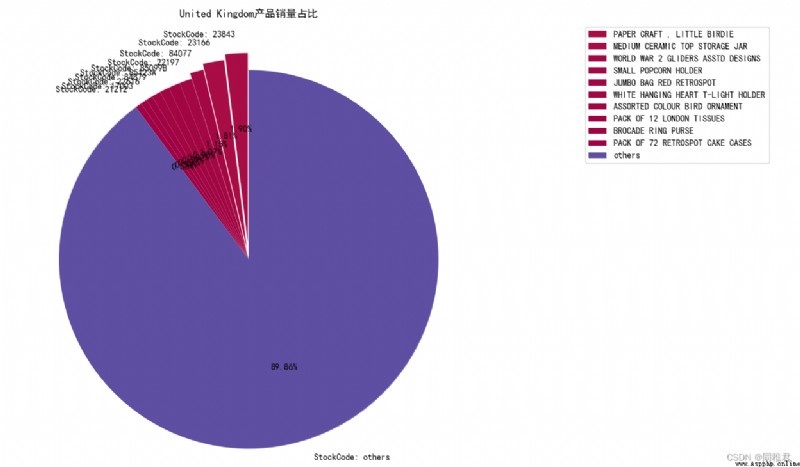
It can be seen that the products of the store are United Kingdom The domestic sales volume is relatively balanced , There is no particularly popular product
Bahrain
The list of products with the top ten sales volume is as follows :


You can see the product “23076” and “23077” The proportion of the sum of sales volume exceeds that of the general , And the numbers of the two products are similar , Explain the product “23076” and “23077” Between Probably There is a strong correlation .
# Load for Apriori Algorithm data
# InvoiceNo: Invoice number . Uniquely assigned to each order 6 An integer . If in letters 'C' start , It means that the order is cancelled .
# StockCode: Product code . Code uniquely assigned to each product .
'''
dataset: Preprocessed data set ;pandas DataFrame
'''
def loatdata(dataset):
dataset["StockCode"] = dataset["StockCode"].apply(lambda x: "," + str(x))
# Group data by invoice number
dataset = dataset.groupby('InvoiceNo').sum().reset_index()
# Put the product code of the same invoice number into the same list
dataset["StockCode"] = dataset["StockCode"].apply(lambda x: [x[1:]])
StockCodeLists = list(dataset["StockCode"])
# Because of this time StockCodeLists The commodity codes with the same invoice number in are combined in a whole string , Therefore, the whole string should be segmented
for i in range(len(StockCodeLists)):
StockCodesString = StockCodeLists[i][0]
StockCodeList = StockCodesString.split(",")
StockCodeLists[i] = StockCodeList
return StockCodeLists
StockCodeLists = loatdata(dataset.loc[:,["InvoiceNo", "StockCode"]])
for item in StockCodeLists:
print(item)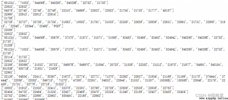
Store in each list “InvoiceNo” The product code of the record with the same invoice number .
from exam import loatdata, dataset
StockCodeLists = loatdata(dataset.loc[:,["InvoiceNo", "StockCode"]])
class Apriori:
# Initialization function , Get the given data set 、 Support threshold 、 Confidence threshold
'''
Function description :
dataset: Given data set ; 2 d list ; Each sub list in the list stores one TID All of the Items
supportThreshold: Support threshold ;float
confidenceThreshold: Confidence threshold ;float
'''
def __init__(self, dataset, supportThreshold, confidenceThreshold):
self.dataset = dataset
self.supportThreshold = supportThreshold
self.confidenceThreshold = confidenceThreshold
'''
Function description :
find 1 Election Anthology C1
param data: Data sets
return: 1 Election Anthology C1
'''
def creatC1(self):
C1 = []
for row in self.dataset:
for item in row:
if [item] not in C1:
C1.append([item])
# Chinese string ascending sort
C1.sort()
# frozenset() return 1 Itemsets , Each item in the itemset is a frozen set , After freezing, no more elements can be added or removed from the collection
return list(map(frozenset, C1))
'''
Function description :
Calculation 1 Support for item candidates , Eliminate itemsets that are less than the minimum support ,
param D: Data sets
param C1: The candidate set
return: return 1 Item frequent sets and their support
'''
def calSupport(self, D, C):
dict_sup = {} # Intermediate storage variables , Used to count
# Iterate over each piece of data , Count each item in the item set
for i in D:
for j in C:
# aggregate j Is it a collection i Subset , If it's a return True, Otherwise return to False
if j.issubset(i):
# Then judge whether there has been any statistics before , If there is no statistics, it is 1
if j not in dict_sup:
dict_sup[j] = 1
else:
dict_sup[j] += 1
# Total number of transactions
sumCount = float(len(D))
# Calculate support , Support = Count of itemsets / Total number of transactions
supportData = {} # Support for storing frequent sets
relist = [] # Used to store frequent sets
for i in dict_sup:
temp_sup = dict_sup[i] / sumCount
# Save the eliminated frequent itemsets and their corresponding support
if temp_sup > self.supportThreshold:
relist.append(i)
supportData[i] = temp_sup
# return 1 Item frequent itemsets and their corresponding support
return relist, supportData
'''
Function description :
Use pruning algorithm , Reduced candidate set space , find k Election Anthology
param Lk: k-1 Item frequent set
param k: The first k term
return: The first k Election Anthology
'''
def aprioriGen(self, Lk, k):
reList = [] # Used to store the second k Election Anthology
lenLk = len(Lk) # The first k-1 Length of term frequent set
# Pairwise traversal
for i in range(lenLk):
for j in range(i + 1, lenLk):
L1 = list(Lk[i])[:k - 2]
L2 = list(Lk[j])[:k - 2]
L1.sort()
L2.sort()
# front k-1 Item equality , Then you can multiply , This can prevent duplicate items
if L1 == L2:
a = Lk[i] | Lk[j] # a by frozenset aggregate
# Pruning
a1 = list(a) # a1 by k An element in the itemset
b = [] # b For all its k-1 Item subset
# structure b: Traversal takes out each element , Convert to set, Successively a1 Remove the element from the , To join the b in
for q in range(len(a1)):
t = [a1[q]]
tt = frozenset(set(a1) - set(t))
b.append(tt)
# When b Are frequent sets , The retention a1, otherwise , Delete
t = 0
for w in b:
# If True, The description belongs to the candidate set , Otherwise, it does not belong to the candidate set
if w in Lk:
t += 1
# If its subsets are frequent sets , be a1 Is a candidate set
if len(b) == t:
reList.append(b[0] | b[1])
return reList
'''
Function description :
Calculate candidates k Item set support , Eliminate candidate sets that are less than the minimum support , Get frequent k Itemsets and their support
param D: Data sets
param Ck: The candidate k Itemsets
return: Return frequently k Itemsets and their support
'''
def scanD(self, D, Ck):
sscnt = {} # Storage support
for tid in D: # Traversing data sets
for can in Ck: # Traverse the candidates
if can.issubset(tid): # Determine whether the data set contains candidate set items
if can not in sscnt:
sscnt[can] = 1
else:
sscnt[can] += 1
# Calculate support
itemNum = len(D) # Total number of transactions
reList = [] # Storage k Item frequent set
supportData = {} # The corresponding support of save frequent sets
for key in sscnt:
support = sscnt[key] / itemNum
if support > self.supportThreshold:
reList.insert(0, key) # If the conditions are met, join Lk in
supportData[key] = support
return reList, supportData
def get_FrequentItemset(self):
# First , find 1 Election Anthology
C1 = self.creatC1()
# Gather the data in each Item The product code in is loaded into the collection , Then put each Items Put it in the list , For support calculation
D = list(map(set, self.dataset))
# Calculation 1 Support for item candidates , Eliminate itemsets that are less than the minimum support , return 1 Item frequent itemsets and their support
L1, supportData = self.calSupport(D, C1)
L = [L1] # Add a list box , bring 1 A frequent set of items is called a single element
k = 2 # k term
# The condition for jumping out of the loop is that there is no candidate set
while len(L[k - 2]) > 0:
# produce k Election Anthology Ck
Ck = self.aprioriGen(L[k - 2], k)
# Calculate candidates k Item set support , Eliminate candidate sets that are less than the minimum support , Get frequent k Itemsets and their support
Lk, supK = self.scanD(D, Ck)
# take supK The key value pairs in are added to supportData In the dictionary
supportData.update(supK)
# Will be the first k The frequent set of items is added to L in
L.append(Lk) # L The last value of is null
k += 1
del L[-1]
# Returns the frequent set and its corresponding support ;L For frequent itemsets , It's a list ,1,2,3 The itemset is an element
return L, supportData
'''
Function description :
Generate all subsets of the set
param fromList:
param totalList:
'''
def getSubset(self, freqList, all_subset):
for i in range(len(freqList)):
t1 = [freqList[i]]
t2 = frozenset(set(freqList) - set(t1)) # k-1 Item subset
if t2 not in all_subset:
all_subset.append(t2)
t2 = list(t2)
if len(t2) > 1:
self.getSubset(t2, all_subset) # All non 1 Item subset
'''
Function description :
Calculate the confidence level , And eliminate the data less than the minimum confidence , The concept of promotion degree is used here
param freqSet: k Item frequent set
param H: k All subsets corresponding to item frequent sets
param supportData: Support
param RuleList: Strong association rules
'''
def calcConf(self, freqSet, all_subset, supportData, strongRuleList):
# Traverse freqSet And calculate the confidence
for conseq in all_subset:
conf = supportData[freqSet] / supportData[freqSet - conseq] # It is equivalent to offsetting the total number of transactions
# Promotion lift Calculation lift=p(a&b)/p(a)*p(b)
lift = supportData[freqSet] / (supportData[conseq] * supportData[freqSet - conseq])
if conf >= self.confidenceThreshold and lift > 1:
print(freqSet - conseq, '-->', conseq, ' Support ', round(supportData[freqSet], 6), ' Degree of confidence :', round(conf, 6),
'lift The value is :', round(lift, 6))
strongRuleList.append((freqSet - conseq, conseq, conf))
'''
Function description :
Generate strong association rules : Frequent itemsets meet the minimum confidence threshold , Strong association rules will be generated
param L: Frequent set
param supportData: Support
return: Return strong association rules
'''
def get_rule(self, L, supportData):
strongRuleList = [] # Store strong association rules
# from 2 The term frequent set begins to calculate the confidence
for i in range(1, len(L)):
for freqSet in L[i]:
freqList = list(freqSet)
all_subset = [] # Storage H1 All subsets of
# Generate all subsets
self.getSubset(freqList, all_subset)
# print(all_subset)
# Calculate the confidence level , And eliminate the data less than the minimum confidence
self.calcConf(freqSet, all_subset, supportData, strongRuleList)
return strongRuleList# Take the Netherlands as an example
Netherlands_dataset = dataset.loc[dataset["Country"]=="Netherlands"]
StockCodeLists2 = loatdata(Netherlands_dataset.loc[:,["InvoiceNo", "StockCode"]])
apriori2 = Apriori(StockCodeLists2, 0.1, 0.7)
L, supportData = apriori2.get_FrequentItemset()
print(" All frequent itemsets :")
for i in range(len(L)):
print(f" frequent {i+1} Itemsets :")
print(f" Number :{len(L[i])}")
for j in L[i]:
print(j)
print(" The association rules that meet the requirements are as follows :")
rule = apriori2.get_rule(L, supportData)
print(f" Number :{len(rule)}")Considering the large amount of data in the data set ( common 392732 strip ), Association rules are sparse , Therefore, the support of association rules in the dataset will be relatively small . After adjusting the support threshold and confidence threshold for many times , Set the support threshold to 0.006, The confidence threshold is 0.7, Generate overall association rules .
Finally get 1069 A frequent 1 Itemsets 、1178 A frequent 2 Itemsets 、529 A frequent 3 Itemsets 、135 A frequent 4 Itemsets 、18 A frequent 5 Itemsets 、1 A frequent 6 Itemsets .
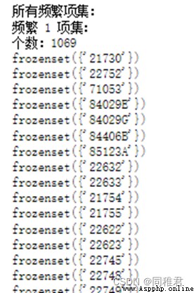
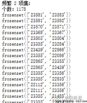
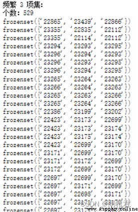
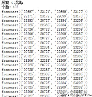
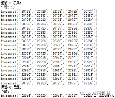
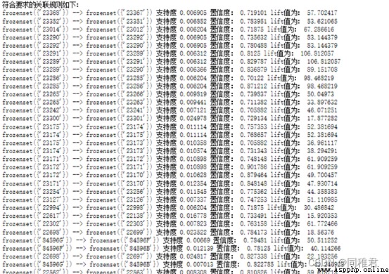
In the frequent item set that meets the confidence threshold , frequent 1 The support of itemsets is generally higher than that of frequent k(1<k<6) Itemsets . A total of 1101 Strong association rules , In all strong association rules , The most supported association rule is :
frozenset({'22697'}) --> frozenset({'22699'}) Support 0.029186 Degree of confidence : 0.782923 lift The value is : 18.534184
'22697' Our product description is :GREEN REGENCY TEACUP AND SAUCER
'22699' Our product description is :ROSES REGENCY TEACUP AND SAUCER
Rank according to the sales volume of products in different countries , Determine the top three countries of product sales as :United Kingdom、Netherlands、EIRE, Then the association rules of these three major countries are analyzed .
①United Kingdom
Set the support threshold to 0.006, The confidence threshold is 0.7.
Get frequent 1 Itemsets 1068 individual 、 frequent 2 Itemsets 1179 individual , frequent 3 Itemsets 571 individual , frequent 4 Itemsets 169 individual , frequent 5 Itemsets 23 individual , frequent 6 Itemsets 1 individual . A total of 1101 Strong association rules .
The three association rules with the highest support are :
frozenset({'22699'}) --> frozenset({'22697'}) Support 0.02859 Degree of confidence : 0.702065 lift The value is : 19.099148
frozenset({'22698'}) --> frozenset({'22697'}) Support 0.024266 Degree of confidence : 0.819473 lift The value is : 22.293137
frozenset({'22698'}) --> frozenset({'22699'}) Support 0.023004 Degree of confidence : 0.776876 lift The value is : 19.07701
②Netherlands
Set the support threshold to 0.1, The confidence threshold is 0.7.
Get frequent 1 Itemsets 34 individual 、 frequent 2 Itemsets 25 individual , frequent 3 Itemsets 8 individual , frequent 4 Itemsets 1 individual . A total of 47 Strong association rules .
The three association rules with the highest support are :
frozenset({'22630'}) --> frozenset({'22629'}) Support 0.221053 Degree of confidence : 0.954545 lift The value is : 3.238636
frozenset({'22326'}) --> frozenset({'22629'}) Support 0.189474 Degree of confidence : 0.72 lift The value is : 2.442857
frozenset({'22630'}) --> frozenset({'22326'}) Support 0.168421 Degree of confidence : 0.727273 lift The value is : 2.763636
③EIRE
Set the support threshold to 0.1, The confidence threshold is 0.7.
Get frequent 1 Itemsets 77 individual 、 frequent 2 Itemsets 45 individual , frequent 3 Itemsets 43 individual , frequent 4 Itemsets 11 individual . A total of 258 Strong association rules .
The three association rules with the highest support are :
frozenset({'22697'}) --> frozenset({'22699'}) Support 0.119231 Degree of confidence : 0.911765 lift The value is : 5.387701
frozenset({'22698'}) --> frozenset({'22699'}) Support 0.103846 Degree of confidence : 0.964286 lift The value is : 5.698052
frozenset({'22698'}) --> frozenset({'22697'}) Support 0.1 Degree of confidence : 0.928571 lift The value is : 7.10084
From the above mining results , You can find itemsets {'22699'}、{'22698'}、{'22697'} stay United Kingdom and EIRE Are frequent itemsets with high support , And these three frequent itemsets are strongly correlated in the sales of these two countries . Considering that Ireland is geographically close to Britain , Therefore, the consumption characteristics of the people are close to , The mining results of association rules also indirectly prove this . The association rules of products purchased by Dutch people are different from those in Britain and Ireland , It is worth noting that the product '22629'、'22630'、'22326' The sales volume in the Netherlands ranked second 、 3、 ... and 、 Five ( The pie chart of the sales volume of products in the Netherlands is as follows ), Explain the products with strong relevance , Its sales volume is often similar , Through the strong relevance of products , Hot selling products can drive the sales of related products .
