One 、 introduction

Univariate linear regression ： There is only one variable involved

Multiple linear regression ： Two or more variables involved

There is a certain error between the predicted result and the real value （ Pictured ）：

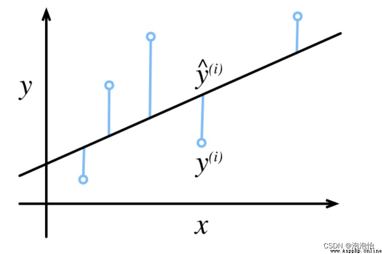
  This article takes y=-2x+8 For example , The method of estimating the regression coefficient by using the least square method and python Realization .

Two 、 Formula derivation

1. Least square method ：

Suppose you know a series of scatter points （xi,yi)

We will （xi,yi) Plug in y =kx+b have to

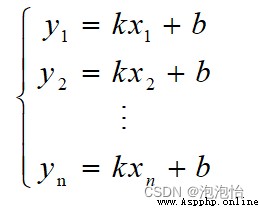
  Construct the least squares function ：

  Yes k and b Calculate the partial derivatives respectively to get ：

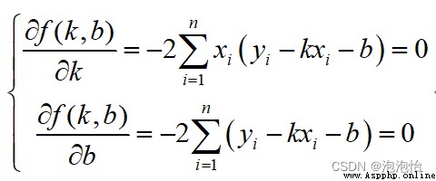
Both ends of the above equations are divided by n have to ：

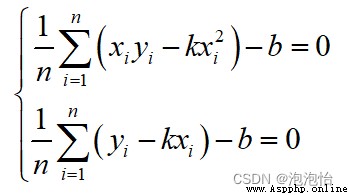
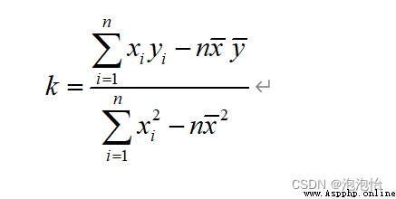
  The coefficient can be obtained by substituting it b.

  3、 ... and 、python Program

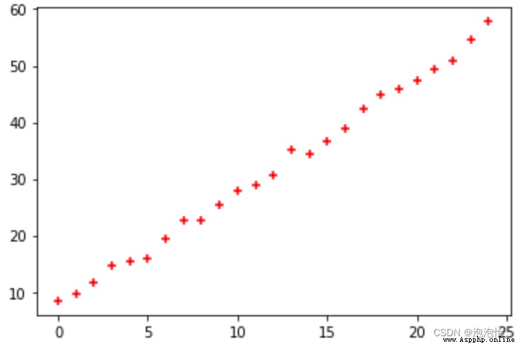
1. Interpret the curve change trend according to the scatter diagram

import numpy as np
import matplotlib.pyplot as plt
%matplotlib inline
trainX=np.arange(25)
trainY=2*trainX+8+np.random.randn(25)
plt.scatter(trainX, trainY,color='red',marker='+')

The result is shown in the figure ：

2. The regression coefficient is calculated as follows ：

n=25
xu=np.sum(trainX)/n
yu=np.sum(trainY)/n
k1 = sum( trainX * trainY ) - n * xu * yu;
k2 = sum( trainX * trainX ) - n * xu * xu;
k = k1 / k2;
b = yu - k * xu;

  give the result as follows ：k=2.0174825107892924, b=7.508028732222016

3. The complete code is as follows

import numpy as np
import matplotlib.pyplot as plt
%matplotlib inline
trainX=np.arange(25)
trainY=2*trainX+8+np.random.randn(25)
plt.scatter(trainX, trainY,color='red',marker='+')
n=25
xu=np.sum(trainX)/n
yu=np.sum(trainY)/n
k1 = sum( trainX * trainY ) - n * xu * yu;
k2 = sum( trainX * trainX ) - n * xu * xu;
k = k1 / k2;
b = yu - k * xu;
Y1=k*trainX+b
fig,ax = plt.subplots()
ax.scatter(trainX, trainY,color='red',marker='+')
ax.plot(trainX, Y1,color='blue')

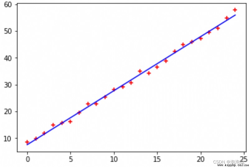
  The result is shown in Fig. ：

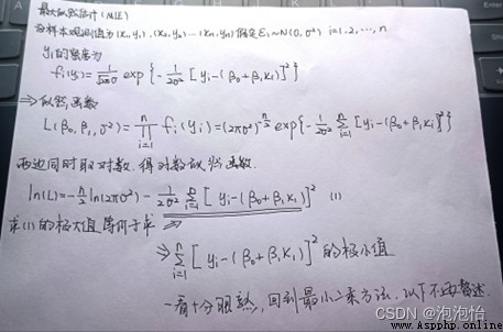
Be careful ： Derivation of additional maximum likelihood estimation ：