One . Preface

        This paper mainly uses neural network to predict handwritten data sets , The data used is still the data of multi classification logistic regression , This time I filled in one more ex3weight.mat file , Yes 5000 Samples ,400 Column eigenvalues

Two . Code parsing

1. Import package

        The package here is the same as that used in multi classification logistic regression

import numpy as np
import matplotlib.pyplot as plt
from scipy.io import loadmat

2. Data import and data initialization

        Here you need to take two files ,ex3data1 Where is the X,y Data set with key ,ex3weights There are two stored in theta matrix , It is used to evolve data in the first and second layers respectively , It also needs to be in X Insert... In the first column of 1

data = loadmat('ex3data1.mat')
# print(data) # View the data
# print(data.keys()) # keyword (['__header__', '__version__', '__globals__', 'X', 'y'])
data_theta = loadmat('ex3weights.mat') # Deposit theta matrix
# print(data_theta) # Look at the data
# print(data.keys()) # View keywords (['__header__', '__version__', '__globals__', 'Theta1', 'Theta2'])
X = data['X']
y = data['y']
X_add1 = np.matrix(np.insert(X, 0, values=np.ones(5000), axis=1)) # Insert 1
y = np.matrix(y)
# print(X_add1.shape,y.shape) # see X_add1,y dimension ---(5000, 401) (5000, 1)
theta1 = np.matrix(data_theta['Theta1'])
theta2 = np.matrix(data_theta['Theta2'])
# print(theta1.shape,theta2.shape) # see theta1,theta2 dimension ()---(25, 401) (10, 26)

ex3weights Data presentation  

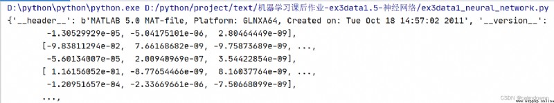
  The first line is x_add1 and y Dimensions , The second line is theta1 and theta2 Dimensions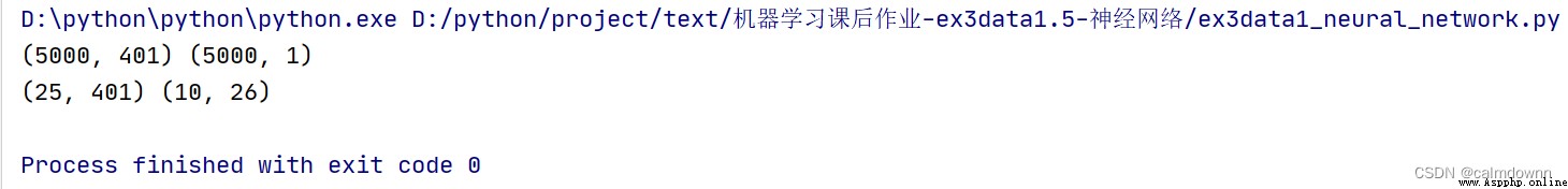

 3.sigmoid function

        There is no explanation here , Almost every time you use

def sigmoid(z):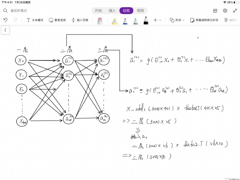
return 1/(1+np.exp(-z))

4. To pass

         Here I draw a simple picture of the process of transmission , If you can't understand it, you can watch it in combination with the teacher's video , The following also describes the changes of matrix dimensions during the transfer process , It's divided into three layers , Each layer has its own evolutionary direction , The last layer gets 10 Probability values , Namely 1-10 Prediction rate of hx（ I forgot to draw one in the picture a0, The second layer also needs to add a column 1）

a1 = X_add1 # first floor （5000*400）
z2 = a1 @ theta1.T
a2 = sigmoid(z2) # Get the second layer matrix （5000*25）
a2 = np.insert(a2, 0, values=1, axis=1) # Insert a column on the second floor 1(5000*26)
# print(a2.shape) # (5000, 26)
z3 = a2 @ theta2.T
a3 = sigmoid(z3) # Get the third layer matrix （5000*10）

5. Prediction function

        The prediction function is roughly the same as that in multiple logistic regression , This time we get the result matrix directly , Just from 5000*10 Find the largest in each row hx, And with y Just compare , It becomes more convenient

# Prediction function
def predict_fuc(a3,y):
p_max = np.argmax(a3,axis=1) # from a3 Find the coordinates of the maximum value in each row in the matrix
p_max_last = np.matrix(p_max.reshape(5000,1) + 1) # Because the subscript returned is 0-9 So add one here to match y comparing
count = 0
for i in range(0,5000):
if p_max_last[i] == y[i]:
count += 1
return count/len(y)
pass

6. Result display  

        It can be seen that the success rate is compared with multi classification logistic regression , A lot of improvement , The running speed is also many times faster , So neural network method is still very practical

print(f' The predicted success rate is {predict_fuc(a3,y) * 100}%')

  3、 ... and . All the code

import numpy as np
import matplotlib.pyplot as plt
from scipy.io import loadmat
data = loadmat('ex3data1.mat')
# print(data) # View the data
# print(data.keys()) # keyword (['__header__', '__version__', '__globals__', 'X', 'y'])
data_theta = loadmat('ex3weights.mat') # Deposit theta matrix
# print(data_theta) # Look at the data
# print(data.keys()) # View keywords (['__header__', '__version__', '__globals__', 'Theta1', 'Theta2'])
X = data['X']
y = data['y']
X_add1 = np.matrix(np.insert(X, 0, values=np.ones(5000), axis=1)) # Insert 1
y = np.matrix(y)
# print(X_add1.shape,y.shape) # see X_add1,y dimension ---(5000, 401) (5000, 1)
theta1 = np.matrix(data_theta['Theta1'])
theta2 = np.matrix(data_theta['Theta2'])
# print(theta1.shape,theta2.shape) # see theta1,theta2 dimension ()---(25, 401) (10, 26)
def sigmoid(z):
return 1/(1+np.exp(-z))
# Prediction function
def predict_fuc(a3,y):
p_max = np.argmax(a3,axis=1) # from a3 Find the coordinates of the maximum value in each row in the matrix
p_max_last = np.matrix(p_max.reshape(5000,1) + 1) # Because the subscript returned is 0-9 So add one here to match y comparing
count = 0
for i in range(0,5000):
if p_max_last[i] == y[i]:
count += 1
return count/len(y)
pass
a1 = X_add1 # first floor （5000*400）
z2 = a1 @ theta1.T
a2 = sigmoid(z2) # Get the second layer matrix （5000*25）
a2 = np.insert(a2, 0, values=1, axis=1) # Insert a column on the second floor 1(5000*26)
# print(a2.shape) # (5000, 26)
z3 = a2 @ theta2.T
a3 = sigmoid(z3) # Get the third layer matrix （5000*10）
print(f' The predicted success rate is {predict_fuc(a3,y) * 100}%')