List of articles

• One . Introduction to data sources
• Two . Use DBSCAN Clustering
• Reference resources ：

One . Introduction to data sources

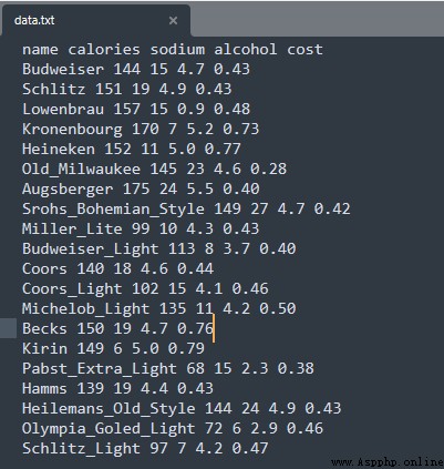
data source :
A beer data source , For the convenience of demonstration , Data only 20 That's ok .

• name The name of beer
• calories The calories of beer
• sodium Na content
• alcohol alcohol content
• cost Price

Two . Use DBSCAN Clustering

Code :

import pandas as pd
from sklearn.cluster import DBSCAN
from pandas.plotting import scatter_matrix
import matplotlib.pyplot as plt
import numpy as np
from sklearn.preprocessing import StandardScaler
from sklearn import metrics
# Read data source 
beer = pd.read_csv('E:/file/data.txt', sep=' ')
X = beer[["calories","sodium","alcohol","cost"]]
# Training data source 
db = DBSCAN(eps=10, min_samples=2).fit(X)
# Tag it 
labels = db.labels_
beer['cluster_db'] = labels
beer.sort_values('cluster_db')
# drawing 
colors = np.array(['red', 'green', 'blue', 'yellow'])
pd.scatter_matrix(X, c=colors[beer.cluster_db], figsize=(10,10), s=100)
plt.show()
# Verify the effect of the model 
score_scaled = metrics.silhouette_score(X,beer.cluster_db)
print(" Use DBSCAN The model effect of :")
print(score_scaled)

Test record :
Use DBSCAN The model effect of :
0.49530955296776086

analysis :
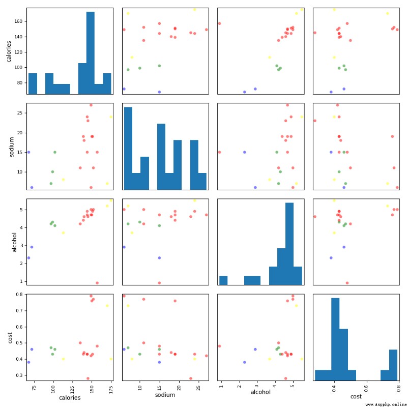
From the perspective of scoring and visualization , Clustering effect is not ideal , Not as good as K-Means effect .
For the complex use of sample sets DBSCAN.
For the sample set, simply use it directly K-Means that will do .

Reference resources ：

1. https://study.163.com/course/introduction.htm?courseId=1003590004#/courseDetail?tab=1