Note source :
Python Data structures and Algorithms Second Edition (runestone There is a free English version );
The teacher is in class ppt;
Learning steps :
1、Python
2、Algorithm
3、Basic Data Structure
you can learn it from
by Python course
Users are equivalent to drivers ;
Our yard farmer is equivalent to the person who assembles the car ;
( Those parts are ADT, We just need to know how to use those parts )
The complex basic work at the bottom : We don't need to know how to make car parts ;

Algorithm: ways to solve things.
A procedural Algorithm Determinants of good and bad
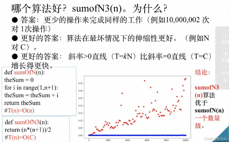
Because we don't know what kind of function to use to model the runtime performance of the algorithm , So this approach did not get a useful measure ; So we need to find algorithm characteristics that are independent of the program or computer used .
Iterative solution function :
def sumOfN(n):
theSum=0
for i in range(1,n+1):
theSum=theSum+i
return theSum
def sumOfN3(n) Using a closed equation
# Calculate without iteration n The sum of return (n*(n+1))/2
ns=np.linspace(10,10_000,100,dtype=int)
ts3=[timeit.timrit('sumOfN3(r)',setup=f'r={
n}',number=1000,globals=globals()) for n in ns]
plt.plot(ns,ts3,'ob')
ps: Testing takes up memory :MemoryMonitor class
sum Drawing function of running time change :
import matplotlib.pyplot as plt
import numpy as np
import timeit
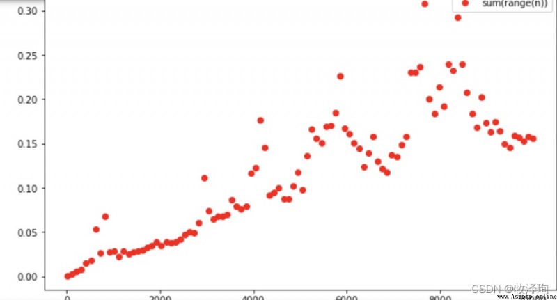
ns=np.linspace(10,10_000,100,dtype=int)# The scale of the problem
ts=[timeit.timeit('sumOfN(r)',setup=f'r={
n}',number=1000,globals=globals())for n in ns]
plt.plot(ns,ts,'or')# The plot : The scale of the problem is horizontal , Time cost is the vertical axis
#ts=[timeit.timeit('sum(r)',setup=f'r=range{n}',number=1000,globals=globals())for n in ns]
total=0
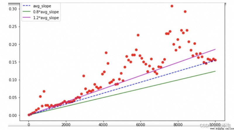
for i in range(len(ns)-1):
total+=(ts[i+1]-ts[i])/(ns[i+1]-ns[i])# Sum of slopes between all adjacent two points
avg_slope=total/(len(ns)-1)
plt.plot(ns,ts,'or')
plt.plot(ns,[avg_slope*n for n in ns],'--b']
# Running time estimation
for n in np.linspace(1,100_000_000,11,dtype=int)
print(f'Rumtime of sum(range({
n:>11,})~{
avg_slope*n/100:>5.2f}s')
>>>>>Runtime of sum(range( 1)~0.00s
>>>>>Runtime of sum(range(10,000,000)~0.08s
degree=100
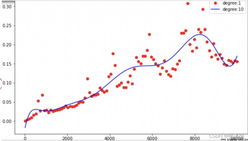
coefffs=np.polyfit(ns,ts,degree)
p=np.ploy1d(coeffs)
pt.plot(ns,ts,'or')
plt.plot(ns,[p(n) for n in ns],'-b')
for n in np.linspace(1,100_000_000,11,dtype=int)
print(f'Rumtime of sum(range({
n:>11,})~{
p(n)/100:2f}s')
>>>>>Runtime of sum(range( 1)~0.00s
>>>>>Runtime of sum(range(10,000,000)~929393014.....s
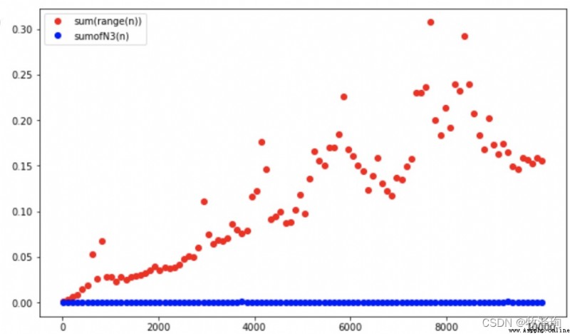
ns=np.linspace(10,10_000,100,dtype=int)
ts=[timeit.timrit('sum(r)',setup=f'r=range({
n})',number=1000,for n in ns]
ts3=[timeit.timeit('sumOfN3(r)',setup=f'r={
n}',number=1000,globals=globals()) for n in ns]
plt.plot(ns,ts,'or')
plt.plot(ns,ts3,'ob')
Algorithm execution time : You can use The number of steps required to solve the problem is expressed (T(n)=S(n))
The scale of the problem :n
T(n): solve n The time spent on the problem
S(n): solve n The steps needed to solve the problem
# Program 1 S(n)=5
i=1 #1
j=2 #1
temp=i #1
i=j #1
j=temp #1
# Program 2
x=0 #1
n=2 #1
for i in range(1,2*n):#️range(a,b) It's from a To b-1
x=x+1#2n-1
S(n)=O(f(n)) : The upper bound of the order of increase in the running time of the algorithm
f(n):S(n) The decisive part of growth

ps: Constant order , Logarithmic order , Linear order , Linear logarithmic order , Square order , Polynomial order , Exponential order , Factorial stage 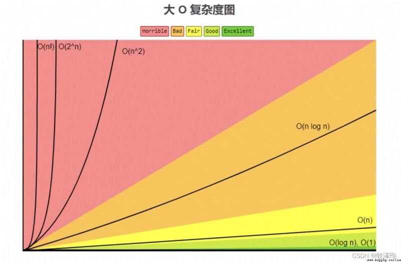
Ps: The complexity of exponential order and factorial order is a difficult problem .
example ( function ):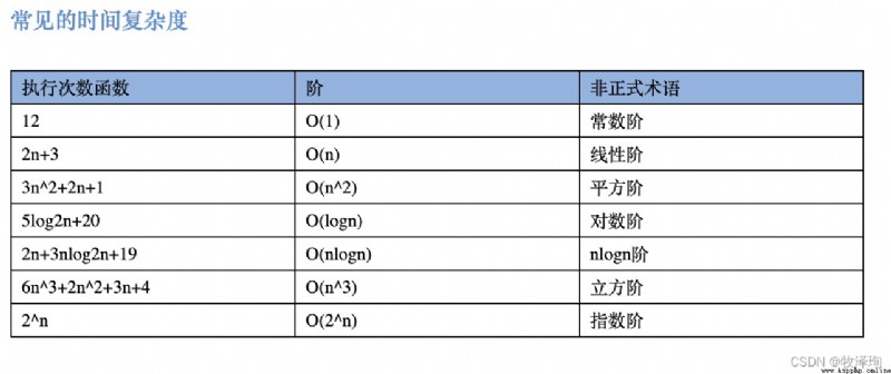
example ( Program ):
f(n):S(n) The fastest growing part
T(n)=O(f(n))=O(n^2)**
# Program 1 s(n)=3+(n-1)+(n-1)*(zn+1) f(n)=S(n) The fastest growing part
y=0 #1 T(n)=O(f(n))=O(n^2)
x=0 #1
n=3 #1
for i in range (1,n):
x=y+1#(n-1)
for j in range(2*n+1)
x=x+1#(2n+1)
# Program 2 s(n)=n^2 T(n)=O(f(n))=O(n^2)
for i in range(n):#n
for j in range(n):#n
M1[i][j]=M1[i][j]+M2[i][j]
The performance of the algorithm sometimes depends not only on the size of the problem ,
It also depends on data values .
Classic word detection problem
1、 use None Replace the same element traversal
Heteronym : One string contains the same elements as another string , But the order is different .
S1[0] stay S2 Traverse , And S2 The elements in are compared in turn until the same appears , take S2 The element in is equal to None.
Every element every time :
2、 Sort the characters in alphabetical order , The result of out of order words will be the same string .
Python in , You can first convert a string into a list , Then use the built-in sort Method to sort the list . At first glance, you may only need to traverse the basic characters once , But it still needs to be considered sort() The price of .
3、 Because characters may have 26 Kind of , So use 26 A counter , Corresponding to each character . Every character encountered , Add the corresponding counter 1.
ord() function :
print(ord(‘5’)) # 53
print(ord(‘A’)) # 65
print(ord(’$’)) # 36
def ang(s1,s2):
c1=[0]*26
c2=[0]*26
for i in range(len(s1)):
pos=ord(s1[i])-ord('a')
print(pos)
c1[pos]=c1[pos]+1
print(c1)
for i in range(len(s2)):
pos=ord(s2[i])-ord('a')
c2[pos]=c2[pos]+1
j=0
Stillok=True
while j<26 and Stillok:
if c1[i]==c2[j]:
j=j+1
print(j)
else:
Stillok=False
return Stillok
ang("za","bdca")
I gave an obvious example :
"za"print(pos)print(c1)
The observation clearly shows pos and c1 The purpose of the counter .
Algorithms of different orders of magnitude
Show algorithms of different orders of magnitude ,
4 Ways of planting
# Tested function
def test1(n):# Connect
l=[]
for i in range(n):
l=l+[i]
def test2(n):# Additional
l=[]
for i in range(n):
l.append(i)
def test3(n):# List parsing
l=[i for i in range(n)]
def test4(n):#range function + List constructor
l=list(range(n))
Compare the efficiency of four ways of constructing lists : mapping time Class function
# The horizontal axis : The scale of the problem n
ns=np.linspace(10,10_00,100,dtype=int)
# The vertical axis : The time cost of solving the problem
lts1=[timeit.timeit('test1(r)',setup=f'r={
n}',number=100,globals=globals()) for n in ns]
lts2=[timeit.timeit('test2(r)',setup=f'r={
n}',number=100,globals=globals()) for n in ns]
lts3=[timeit.timeit('test3(r)',setup=f'r={
n}',number=100,globals=globals()) for n in ns]
lts4=[timeit.timeit('test4(r)',setup=f'r={
n}',number=100,globals=globals()) for n in ns]
# Draw function 1-4 The scale of the problem n Function corresponding to time cost
plt.plot(ns,lts1,'sb')
plt.plot(ns,lts2,'g')
plt.plot(ns,lts3,'r')
plt.plot(ns,lts4,'K')
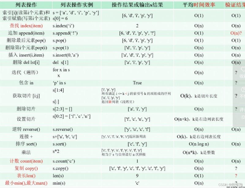
POP
# function
popzero=timeit.Timer("x.pop(0)","from_main_import x")# From the list header pop Out , To traverse the list
popend=timeit.Timer("x.pop()","from_main_import x")# From the end of the list pop Out , It has nothing to do with length
# The vertical axis : Time cost
popendtime=[]
popzerotime=[]
for i in range(10000,1000001,100):
x=list(range(i))
pop_end_t = pop_end.timeit(number=1000)
popendtime.append(pop_end_t)# Insert using timeit Function to calculate the time cost array
x = list(range(i))
pop_zero_t = pop_zero.timeit(number=1000)
popzerotime.append(pop_zero_t)# Insert using timeit Function to calculate the time cost array
# The horizontal axis :
ns=np.linspace(10000,1000001,100,dtype=int)
plt.plot(ns,popendtime,'sb')
plt.plot(ns,popzerotime,'dr')
index(x) lookup
# function
index=timeit.Timer("lst.index(x)","from_main_import lst,x")
# The vertical axis : Time cost
indextime=[]
for n in range(1000,100001,1000):
lst=list(range(n))
x=n//2
index_t=index.timeit(number=1000)
indextime.append(index_t)# Insert using timeit Function to calculate the time cost array
# The horizontal axis :
ns=np.linspace(1000,100000,100,dtype=int)
plt.plot(ns,indextime,'.g',label='index')
plt.lengend()
insert(i,x)
# function
insert=timeit.Timer("lst.index(i,x)","from_main_import lst1,x")
# The vertical axis : Time cost
inserttime=[]
for n in range(1000,100001,1000):
lst1=list(range(n))
i=0
x=0
insert_t=insert.timeit(number=1000)
inserttime.append(insert_t)# Insert using timeit Function to calculate the time cost array
# The horizontal axis :
ns=np.linspace(1000,100000,100,dtype=int)
plt.plot(ns,insertime,'.b',label='insert')
plt.lengend()
remove(x)
remove=timeit.Timer("lst2.remove(x)","from_main_import lst2,x")
del lst[i]
delete=timeit.Timer("del lst3a[i][0];i=i+1","from_main_import lst3a,i")
sort()
sort=timeit.Timer("lst4.reverse()","from_main_import lst4")
reverse()
reverse=timeit.Timer("lst5.reverse()","from_main_import lst5")
count(x)
count=timeit.Timer("lst6.count(x)","from_main_import lst6,x")
append(x)
append=timeit.Timer("lst7a[i].append(0);i+=","from_main_import lst7a,i")
List index assignment operation [ ]
# function
idexassign=timeit.Timer("lst8[i]=0)","from_main_import lst8,i")
# The vertical axis : Time cost
idxassigntime=[]
for n in range(10000,1000001,10000):
lst1=list(range(n))
i=n//2
idxa_t=idxassign.timeit(number=1000)
inserttime.append(idxa_t)# Insert using timeit Function to calculate the time cost array
# The horizontal axis :
ns=np.linspace(10000,1000001,100,dtype=int)
plt.plot(ns,idxassigntime,'.','color='darkorange',
label='insert')
plt.lengend()
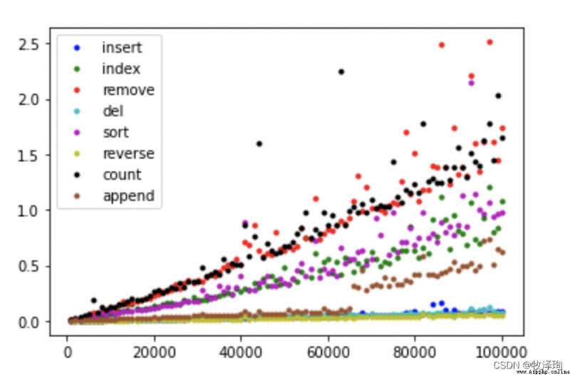
Time comparison to judge whether random numbers exist in lists and dictionaries
import timeit
import random
# Definition An array of storage times
lst_timelst=[]
d_timelst=[]
for i in range((10000, 1000001, 20000):
t=timeit.Timer("random.randrange(%d)in x"%i,"from_main_import random,x")
x=list(range(i))# List constructor
list_time=t.timeit(number=1000)
# The time cost of storing the list array
lst_timelst.append(list_time)
x={
j:None for j in range(i))
d_time=t.timeit(number=1000)# Dictionary construction
# The time cost of storing the dictionary array
d_timelst.append(d_time)
#drawing the curve
plt.plot(ns,lst_timelst,'.b',label='list')# list
plt.plot(ns,d_timelst,'.r',label='dict')# Dictionaries
# I have no write output operation