Catalog
One 、 What is? Q learning Algorithm ?
1.Q table
2.Q-learning Algorithm pseudocode
Two 、Q-Learning solve TSP Of python Realization
1) Problem definition
2) establish TSP Environmental Science
3) Definition DeliveryQAgent class
4) Define each episode Next agent The process of learning
5) Define the main function of training
6) experimental result
1. The environment create
2. Instantiation agent class
3.agent Train to learn
Q-learning The algorithm is very suitable for beginners to understand reinforcement learning , It is the easiest to code and understand . Q-learning Algorithm is a kind of model-free、off-policy/value_based Reinforcement learning algorithm , That is, it does not consider the characteristics of the environment , adopt Q Function to find the optimal action selection strategy .Q value (action value function) It calculates the future reward expectation for taking the action in the current state , The formula is derived as follows :
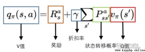

For more basic principles and concepts of reinforcement learning, see Reinforcement learning series ( One ): Basic principles and concepts
Q representative quality, That is, the quality of the action . Create a table Q, take state-action-Q Estimates are stored , By retrieving Q surface , Can get in the current state Select each action An estimate of future reward expectations that can be obtained ,Q-learning The core of is to keep updating Q The table gives a better and better approximation .

Step one : Create and initialize a action-space*state space The size of Q surface , Generally, initialization sets all values to 0;
Step two : Into the loop , Until the iteration condition is reached :
Step three : retrieval Q surface , In current state s Next basis Q The estimated value of and Policy Select a action a;
Step four : perform action a, retrieval Q surface , State transferred to  Corresponding Q The maximum value plus the real-time reward for this action reward It's state s The true value of value ;
Step five : Update according to Behrman equation Q surface .
that , At the beginning of the Q Values are 0, How do we choose the next action ? This time reflects Policy The importance of , A common practice is to introduce a parameter  , The value is 0-1 Between ,
 Embodies the exploration / utilize (exploration/exploitation) Trade off .
 The bigger it is , Randomness / The more exploratory , Usually initially
  Close to or equal to 1 Randomly choose the next action for a lot of exploration ; With agent Keep learning , Yes Q Our estimate is getting more and more accurate , We will gradually reduce
  Value , Rely more on current Q value .
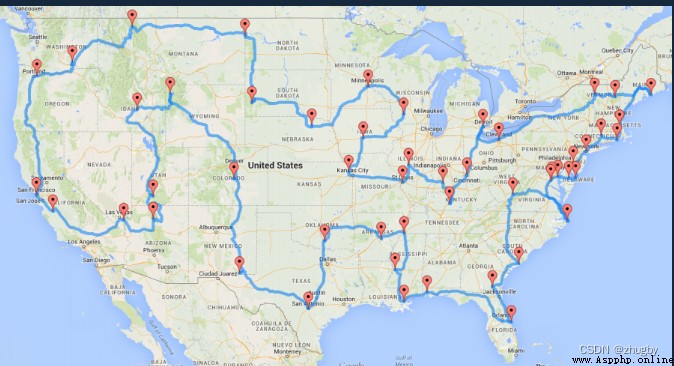
Travel agent problem ( TSP) It is a typical optimization problem , The purpose is to find the shortest way to visit each city . To use RL How to solve this problem TSP problem , We need to TSP Problem into RL problem , Definition RL Elements of :
agent: The delivery man ;
environment: The goods to be delivered and the location of the city node to be visited ;
state: The city node of the current deliveryman ;
action: Decisions to be made at each node , Which node to go to next ;
reward: Real time rewards , How far is the distance between two nodes .
RL The goal of goal Is making reward The sum of is the largest , That is, the shortest distance of the access route .
stay python Create a simple TSP The environment is very simple , Specify the number of city nodes , Randomly generate city node coordinates ; And calculate the distance between different cities as reward value .python The specific implementation code is as follows , Created a DeliveryEnvironment class , The default number of city nodes is 10 individual , Randomly select a node as the starting point , Define a function display for drawing TSP Of Environment.
# Import required packages
import pandas as pd
import numpy as np
import matplotlib.pyplot as plt
import os
import time
from tqdm import tqdm_notebook
from scipy.spatial.distance import cdist
import imageio
from matplotlib.patches import Rectangle
from matplotlib.collections import PatchCollection
plt.style.use("seaborn-dark")
import sys
sys.path.append("../")
from rl.agents.q_agent import QAgent
class DeliveryEnvironment(object): # Initialization environment
def __init__(self,n_stops = 10,max_box = 10,method = "distance",**kwargs):
print(f"Initialized Delivery Environment with {n_stops} random stops")
print(f"Target metric for optimization is {method}")
# Parameter initialization
self.n_stops = n_stops
self.action_space = self.n_stops
self.observation_space = self.n_stops
self.max_box = max_box
self.stops = []
self.method = method
# Generate city nodes
self._generate_constraints(**kwargs)
self._generate_stops()
self._generate_q_values()
self.render()
# Initialization environment
self.reset()
def _generate_stops(self): # Generate city nodes
# Generate geographical coordinates
xy = np.random.rand(self.n_stops,2)*self.max_box # Generate customer point coordinates
self.x = xy[:,0]
self.y = xy[:,1]
def _generate_q_values(self,box_size = 0.2): # Calculate the distance between different nodes to act as reward
# Generate actual Q Values corresponding to time elapsed between two points
if self.method in ["distance"]:
xy = np.column_stack([self.x,self.y])
self.q_stops = cdist(xy,xy) # Calculate the distance matrix to act as reward
else:
raise Exception("Method not recognized")
# Drawing function
def render(self,return_img = False):
fig = plt.figure(figsize=(7,7))
ax = fig.add_subplot(111)
ax.set_title("Delivery Stops")
# Show stops
ax.scatter(self.x,self.y,c = "red",s = 50)
# Show START
if len(self.stops)>0:
xy = self._get_xy(initial = True) # The first point generated as start spot , The text position is xy[1]-0.05
xytext = xy[0]+0.1,xy[1]-0.05
ax.annotate("START",xy=xy,xytext=xytext,weight = "bold")
# Show itinerary
if len(self.stops) > 1:
ax.plot(self.x[self.stops],self.y[self.stops],c = "blue",linewidth=1,line)
# The end of the path should return to the starting point
xy = self._get_xy(initial = False)
xytext = xy[0]+0.1,xy[1]-0.05
ax.annotate("END",xy=xy,xytext=xytext,weight = "bold")
if hasattr(self,"box"):
left,bottom = self.box[0],self.box[2]
width = self.box[1] - self.box[0]
height = self.box[3] - self.box[2]
rect = Rectangle((left,bottom), width, height)
collection = PatchCollection([rect],facecolor = "red",alpha = 0.2)
ax.add_collection(collection)
plt.xticks([])
plt.yticks([])
if return_img:
# From https://ndres.me/post/matplotlib-animated-gifs-easily/
fig.canvas.draw_idle()
image = np.frombuffer(fig.canvas.tostring_rgb(), dtype='uint8')
image = image.reshape(fig.canvas.get_width_height()[::-1] + (3,))
plt.close()
return image
else:
plt.show()
# Reset to the next iteration
def reset(self):
# Stops placeholder
self.stops = []
# Random first stop
first_stop = np.random.randint(self.n_stops) # Randomly generate the first initial node
self.stops.append(first_stop)
return first_stop
# according to reward Select the next action
def step(self,destination):
# Get current state Get the current state
state = self._get_state()
new_state = destination
# Get reward for such a move Every action obtain reward
reward = self._get_reward(state,new_state)
# Append new_state to stops Go to the next state
self.stops.append(destination)
done = len(self.stops) == self.n_stops
return new_state,reward,done
# Get the current state That is, the currently arrived node location
def _get_state(self):
return self.stops[-1]
# Get each coordinate X and Y value
def _get_xy(self,initial = False):
state = self.stops[0] if initial else self._get_state()
x = self.x[state]
y = self.y[state]
return x,y
# Definition reward function
def _get_reward(self,state,new_state): #
base_reward = self.q_stops[state,new_state] #base_reward Is the distance between two nodes
if self.method == "distance":
return base_reward
@staticmethod
def _calculate_point(x1,x2,y1,y2,x = None,y = None):
if y1 == y2:
return y1
elif x1 == x2:
return x1
else:
a = (y2-y1)/(x2-x1)
b = y2 - a * x2
if x is None:
x = (y-b)/a
return x
elif y is None:
y = a*x+b
return y
else:
raise Exception("Provide x or y")
Decide to select the next node Policy, Randomly produce a 0-1 Between the value of the , If you compare  Big , choice Q The most valuable action, Otherwise, randomly select an unreached node to access .
class DeliveryQAgent(QAgent):
def __init__(self,*args,**kwargs):
super().__init__(*args,**kwargs)
self.reset_memory()
def act(self,s):
# Get Q Vector copyq surface
q = np.copy(self.Q[s,:])
# Avoid already visited states Shield the nodes that have passed This place should be able to add constraints to play mask The role of some nodes
q[self.states_memory] = -np.inf
if np.random.rand() > self.epsilon:
a = np.argmax(q)
else:
a = np.random.choice([x for x in range(self.actions_size) if x not in self.states_memory])
return a
def remember_state(self,s):
self.states_memory.append(s)
def reset_memory(self):
self.states_memory = []Each iteration requires the environment reset To the initial state , Randomly select a node as the initial node , And then according to Policy Continue to select the next node and update Q value .
# every last episode Learning functions
def run_episode(env,agent,verbose = 1):
s = env.reset()
agent.reset_memory()
max_step = env.n_stops
episode_reward = 0
i = 0
while i < max_step: # Number of nodes
# Remember the states Store the points that have been passed
agent.remember_state(s)
# Choose an action Select a action
a = agent.act(s)
# Take the action, and get the reward from environment Get one reward
s_next,r,done = env.step(a)
# Tweak the reward The minus sign minimization problem becomes the maximization problem
r = -1 * r
if verbose: print(s_next,r,done)
# Update our knowledge in the Q-table to update reward stay Q In the table
agent.train(s,a,r,s_next)
# Update the caches Add up reward
episode_reward += r
s = s_next
# If the episode is terminated
i += 1
if done:
break
return env,agent,episode_reward
In the imported QAgent.py Update is defined in Q The function of value is as follows , That is, Behrman formula , Usually epsilon_decay Less than 1, That is, with the continuous learning , The value of is decreasing , Exploratory reduction .
def train(self,s,a,r,s_next):
self.Q[s,a] = self.Q[s,a] + self.lr * (r + self.gamma*np.max(self.Q[s_next,a]) - self.Q[s,a])
if self.epsilon > self.epsilon_min:
self.epsilon *= self.epsilon_decayAnd output the dynamic graph of the training process and the iterative training process reward It's worth changing .
# The function of model training
def run_n_episodes(env,agent,name="training.gif",n_episodes=1000,render_each=10,fps=10): # Training 1000 Time ,10 Draw the picture once
# Store the rewards Store next reward And graphics
rewards = []
imgs = []
# Experience replay
for i in tqdm_notebook(range(n_episodes)):
# Run the episode Iterative learning
env,agent,episode_reward = run_episode(env,agent,verbose = 0)
rewards.append(episode_reward)
if i % render_each == 0:
img = env.render(return_img = True)
imgs.append(img)
# Show rewards Draw reward Change trend of
plt.figure(figsize = (15,3))
plt.title("Rewards over training")
plt.plot(rewards)
plt.show()
# Save imgs as gif
imageio.mimsave(name,imgs,fps = fps) # Output dynamic diagram ,fps Is the frame rate ( Number of frames played per second )
return env,agentCall the classes and functions defined above , Now we simply realize a scale of 500 A travel agent TSP problem .
The designated scale is 500, Selected measures reward Approach is to distance;
env = DeliveryEnvironment(n_stops = 500,method = "distance") # Random generation 500 Nodes The output environment is as follows :
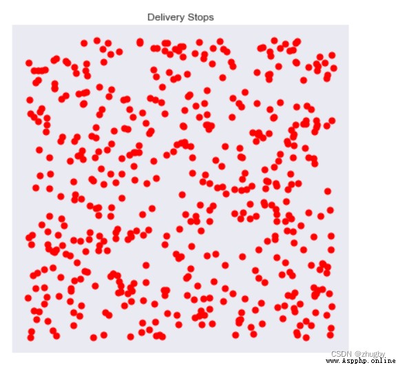
You can also visualize the path by drawing lines between each passing node , Distance to the first few points of the path :
for i in [0,1,2,3]: # Draw the path to follow in the next few steps
env.step(i)
env.render()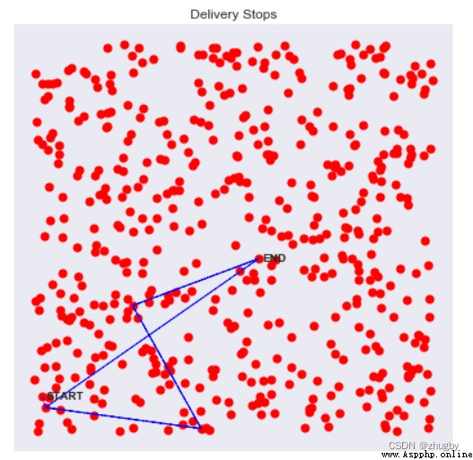
agent = DeliveryQAgent(env.observation_space,env.action_space) #env.observation_space and action_space It is the number of nodes Default iterative learning 1000 Time , You can change ; Record the time of training .
start=time.time()
run_n_episodes(env,agent,"training_500_stops.gif") # Training 1000 Time reward Change trend of front 400 This is basically a random selection of a node to walk , The experience of walking before is used later ,Q What is not in the table is set reward, Some will be updated
end=time.time()
print(' The elapsed time ',end-start)
Model output reward The change trend and running time are as follows :

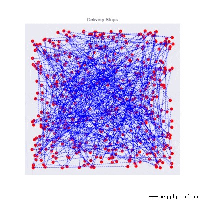
front 400 Sub iteration , Basically, they are exploring new and different routes , It's very random ;400 After the second iteration ,agent Start using what you have learned , Less and less to take random action, but tend to choose Q Worth the most action ;800 It basically converges to an acceptable route from about times .
The dynamic graph of the iterative training process can also reflect the beginning of chaotic continuous exploration and then tend to converge to an acceptable route .
