Inspiration comes from G. Galperin The paper of PLAYING POOL WITH π (THE NUMBER π FROM A BILLIARD POINT OF VIEW),DOI: 10.1070/RD2003v008n04ABEH000252. Here I just briefly introduce the principle , Interested students can read carefully by themselves . The thesis is in English , You can send me a private letter if you need , I'll help you answer any questions .Youtube On 3Blue1Brown There is a video about this paper , There are good pictures and explanations , Better understanding .
In a nutshell ,Galperin My idea is amazing . Different from ordinary calculation π Methods ( Such as infinite series method ), The author uses the conservation of momentum and kinetic energy to calculate π π π!
First , Let's understand the conservation of momentum and energy .
In completely elastic collisions , After the collision, two objects have no other energy consumption except the conversion of kinetic energy . This is the momentum conservation formula of completely elastic collision :
m 1 v 1 + m 2 v 2 = m 1 v 1 ′ + m 2 v 2 ′ m_{1}v_{1}+m_{2}v_{2}=m_{1}v_{1}^{'}+m_{2}v_{2}^{'} m1v1+m2v2=m1v1′+m2v2′
Based on this , The relationship between the two energies can be expressed by the conservation of kinetic energy :
1 2 m 1 v 1 2 + 1 2 m 2 v 2 2 = 1 2 m 1 v 1 ′ 2 + 1 2 m 2 v 2 ′ 2 \frac{1}{2}m_{1}v_{1}^{2}+\frac{1}{2}m_{2}v_{2}^{2}=\frac{1}{2}m_{1}v_{1}^{'2}+\frac{1}{2}m_{2}v_{2}^{'2} 21m1v12+21m2v22=21m1v1′2+21m2v2′2
Connect the above two formulas , We get :
{ m 1 v 1 + m 2 v 2 = m 1 v 1 ′ + m 2 v 2 ′ 1 2 m 1 v 1 2 + 1 2 m 2 v 2 2 = 1 2 m 1 v 1 ′ 2 + 1 2 m 2 v 2 ′ 2 \left\{ \begin{array}{lr} m_{1}v_{1}+m_{2}v_{2}=m_{1}v_{1}^{'}+m_{2}v_{2}^{'} & \\ \\ \frac{1}{2}m_{1}v_{1}^{2}+\frac{1}{2}m_{2}v_{2}^{2}=\frac{1} {2}m_{1}v_{1}^{'2}+\frac{1}{2}m_{2}v_{2}^{'2} & \end{array} \right. ⎩⎨⎧m1v1+m2v2=m1v1′+m2v2′21m1v12+21m2v22=21m1v1′2+21m2v2′2
Simplify the formula , We get :
{ v 1 ′ = ( m 1 − m 2 ) v 1 + 2 m 2 v 2 m 1 + m 2 v 2 ′ = ( m 2 − m 1 ) v 2 + 2 m 1 v 1 m 1 + m 2 \left\{ \begin{array}{lr} v_{1}^{'}=\frac{(m_{1}-m_{2})v_{1}+2m_{2}v_{2}}{m_{1}+m_{2}} & \\ \\ v_{2}^{'}=\frac{(m_{2}-m_{1})v_{2}+2m_{1}v_{1}}{m_{1}+m_{2}} & \end{array} \right. ⎩⎪⎨⎪⎧v1′=m1+m2(m1−m2)v1+2m2v2v2′=m1+m2(m2−m1)v2+2m1v1
such , We have the core algorithm of program simulation .
The ideal physical system shown in the figure below ( No friction , The quality of wall and ground is infinite , The sphere has no angular momentum, etc ) in , These two relationships hold :( Picture source :Galperin)
Specific mathematical proof ,Galperin It is mentioned in the paper . What we have to do , Is to use violent simulation to verify his conclusion . Let the speed of the object move towards the wall be positive , Away from the wall, the speed is negative . The collision between the two occurs in the following cases : 0 > v 2 ≥ v 1 0>v_{2}\geq v_{1} 0>v2≥v1, Two objects will not meet again .
Galperin The mathematical argument of is very detailed . To make a long story short , He proved the following relationship :
Π ( N ) = 314159265358979... Π(Ν)=314159265358979... Π(N)=314159265358979...
among Π ( N ) Π(Ν) Π(N) When the weight of a large object is that of a small object 10 0 N 100^Ν 100N Times the number of collisions , N N N It's calculation π π π Number of digits -1.
What we have to do , Is to write a program based on his thesis .
#!/usr/local/bin/python3
import time
from decimal import *
from decimal import Decimal as dcm # This library improves the precision of floating point operation
getcontext().prec = 50 # The decimal places are set to 50 position
N = int(input("Enter N:"))
m = dcm(1) # initialization m1
M = dcm(m*100**N) # initialization m2
vm0 = dcm(0) # initialization v1
vM0 = dcm(10000) # initialization v2
vm = vm0 # initialization v1'
vM = vM0 # initialization v2'
cnt = -3 # Initialize counter After testing, the software will always count more times So first -3
start = time.time() # Set a timer , Calculate the time required
while not (vm < vM and vM < dcm(0)): # That is, when two objects do not turn right at the same time and no longer meet
vm = dcm((m-M)*vm0+2*M*vM0)/dcm(M+m)
vM = dcm((M-m)*vM0+2*m*vm0)/dcm(M+m) # The two core simulation algorithms mentioned above
cnt += 1
vm0 = dcm(-vm) # Elastic collision , The momentum of a small object becomes in the opposite direction
vM0 = dcm(vM) # Momentum update of large objects , Direction unchanged
cnt += 1 # Hit again
end = time.time() # End timer
print("Number of collisions:", cnt)
print("Time elapse:", end-start, "seconds.") # Output
See the following table for the operation results :( Self made )
The first left column is N Value
The second column is the number of collisions output
The third column is the running time
The fourth column is calculated from the output π π π value
The fifth column is and reality π π π Value gap 
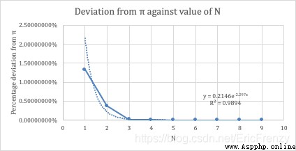
The picture below is N Exponential regression between the change of and the calculation deviation :( Self made by the author )
Visible from above , With N The increase of , The calculated pi exponentially tends to be infinitely accurate .
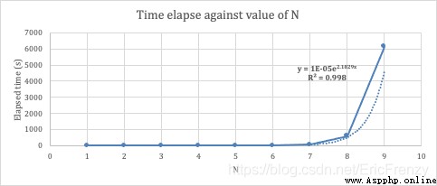
The picture below is N Exponential regression between the change of and the time required for calculation :( Self made by the author )
so , With the exponential improvement of accuracy , The time complexity of calculation is also exponentially increased . therefore , Ordinary notebooks are really not too big N.
Our program is really very effective . However , There are many other calculations π π π The method is more efficient . There are also some omissions in our program . such as , The output value is always odd . This is because in the while The default minimum increment in the loop is 2. Interested partners can think about how to solve ! Maybe we can add a few more judgments ?
about Galperin If you are interested in the thesis, please send me a private message or leave a comment , I will be happy to help you answer relevant questions !
ps: I am using these things to write essays , So please quote !