RIGHT Example:
names = [' The Monkey King ', ' Li Yuanfang ', ' White ', ' Judge dee ', ' dharma ']
courses = [' Chinese language and literature ', ' mathematics ', ' English ']
import random
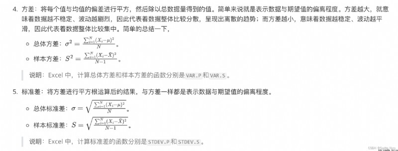
scores = [[random.randrange(60, 101) for _ in range(3)] for _ in range(5)]
print(scores)
# [[100, 97, 76], [91, 79, 66], [84, 78, 71], [87, 81, 96], [73, 71, 88]]
def mean(nums):
""" Calculating mean """
return sum(nums) / len(nums)
def variance(nums):
""" Variance estimation """
mean_value = mean(nums)
return mean([(num - mean_value) ** 2 for num in nums])
def stddev(nums):
""" Find standard deviation """
return variance(nums) ** 0.5
# Count the average score of each student
for idx, name in enumerate(names):
temp = scores[idx]
avg_score = mean(temp)
print(f'{
name} The average score of the exam is :{
avg_score:.1f} branch ')
''' The average score of the monkey king test is :91.0 branch Liyuanfang's average score in the exam is :78.7 branch The average score of the Baiqi test is :77.7 branch The average score of Di Renjie in the exam is :88.0 branch The average score of Dharma test is :77.3 branch '''
# Count the highest scores of each course 、 Lowest score 、 Standard deviation
for idx, course in enumerate(courses):
temp = [scores[i][idx] for i in range(len(names))]
max_score, min_score = max(temp), min(temp)
print(f'{
course} Highest score :{
max_score} branch ')
print(f'{
course} Lowest score :{
min_score} branch ')
print(f'{
course} Standard deviation of grades :{
stddev(temp):.1f} branch ')
''' The highest score in Chinese :100 branch The lowest score in Chinese :73 branch Standard deviation of Chinese achievement :8.8 branch The highest score in Mathematics :97 branch The lowest score in mathematics :71 branch Standard deviation of math scores :8.6 branch The highest score in English :96 branch Minimum score in English :66 branch Standard deviation of English performance :11.1 branch '''
# Output the students and their test scores in the form of lines ( Sort by average from high to low )
results = {
name: temp for name, temp in zip(names, scores)}
sorted_keys = sorted(results, key=lambda x: mean(results[x]), reverse=True)
for key in sorted_keys:
verbal, math, english = results[key]
print(f'{
key}:\t{
verbal}\t{
math}\t{
english}')
''' The Monkey King : 100 97 76 Judge dee : 87 81 96 Li Yuanfang : 91 79 66 White : 84 78 71 dharma : 73 71 88 '''
Python Three artifact of data analysis
import numpy as np
import pandas as pd
import matplotlib.pyplot as plt
# take list Processing into ndarray object
scores = np.array(scores)
print(scores)
''' array([[100, 97, 76], [ 91, 79, 66], [ 84, 78, 71], [ 87, 81, 96], [ 73, 71, 88]]) '''
# View data type
type(scores)
# numpy.ndarray
# Press horizontal ( Student ) averaging
np.round(scores.mean(axis=1), 1)
# array([91. , 78.7, 77.7, 88. , 77.3])
# Press vertical ( Discipline ) Get the highest score 、 Lowest score 、 Standard deviation
scores.max(axis=0)
# array([100, 97, 96])
scores.min(axis=0)
# array([73, 71, 66])
np.round(scores.std(axis=0), 1)
# array([ 8.8, 8.6, 11.1])
scores_df = pd.DataFrame(data=scores, columns=courses, index=names)
scores_df
design sketch :
# Calculate the average score
np.round(scores_df.mean(axis=1), 1)
''' The Monkey King 91.00000 Li Yuanfang 78.66875 White 77.66875 Judge dee 88.00000 dharma 77.33125 dtype: float64 '''
# Add average columns to the table
scores_df[' average ']= scores_df.mean(axis=1)
scores_df
design sketch :
# write in Excel file
scores_df.to_excel(' Test results .xlsx')
# Change plt typeface
plt.rcParams['font.sans-serif'] = ['KaiTi']
plt.rcParams['axes.unicode_minus'] = False
# Change the generated graph to vector graph
%config InlineBackend.figure_format='svg'
# Generate a histogram
scores_df.plot(kind='bar', y=[' Chinese language and literature ',' mathematics ',' English '])
# The scale of the horizontal axis of rotation
plt.xticks(rotation=0)
# Save the chart
plt.savefig(' Score bar .svg')
# Show chart
plt.show()
design sketch :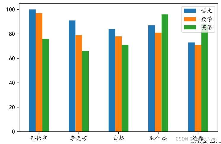
# Get the highest score in the subject 、 Lowest score 、 average
scores_df.max()
''' Chinese language and literature 100.0 mathematics 97.0 English 96.0 average 91.0 dtype: float64 '''
scores_df.min()
''' Chinese language and literature 73.0 mathematics 71.0 English 66.0 average 77.3 dtype: float64 '''
scores_df.std()
''' Chinese language and literature 9.874209 mathematics 9.602083 English 12.361230 average 6.461656 dtype: float64 '''
# Method 1 : adopt array Function will list Processing into ndarray object
array1 = np.array([1, 2, 10, 20, 100])
array1
# array([ 1, 2, 10, 20, 100])
type(array1)
# numpy.ndarray
# Method 2 : Specify a range to create an array object
array2 = np.arange(1, 100, 2)
array2
''' array([ 1, 3, 5, 7, 9, 11, 13, 15, 17, 19, 21, 23, 25, 27, 29, 31, 33,35, 37, 39, 41, 43, 45, 47, 49, 51, 53, 55, 57, 59, 61, 63, 65, 67, 69, 71, 73, 75, 77, 79, 81, 83, 85, 87, 89, 91, 93, 95, 97, 99]) '''
# Method 3 : Specify the range and the number of elements to create an array object
array3 = np.linspace(-5, 5, 101)
array3
''' array([-5. , -4.9, -4.8, -4.7, -4.6, -4.5, -4.4, -4.3, -4.2, -4.1, -4. , -3.9, -3.8, -3.7, -3.6, -3.5, -3.4, -3.3, -3.2, -3.1, -3. , -2.9, -2.8, -2.7, -2.6, -2.5, -2.4, -2.3, -2.2, -2.1, -2. , -1.9, -1.8, -1.7, -1.6, -1.5, -1.4, -1.3, -1.2, -1.1, -1. , -0.9, -0.8, -0.7, -0.6, -0.5, -0.4, -0.3, -0.2, -0.1, 0. , 0.1, 0.2, 0.3, 0.4, 0.5, 0.6, 0.7, 0.8, 0.9, 1. , 1.1, 1.2, 1.3, 1.4, 1.5, 1.6, 1.7, 1.8, 1.9, 2. , 2.1, 2.2, 2.3, 2.4, 2.5, 2.6, 2.7, 2.8, 2.9, 3. , 3.1, 3.2, 3.3, 3.4, 3.5, 3.6, 3.7, 3.8, 3.9, 4. , 4.1, 4.2, 4.3, 4.4, 4.5, 4.6, 4.7, 4.8, 4.9, 5. ]) '''
# Method four : Create an array object by randomly generating elements
# Random decimal
array4 = np.random.random(10)
array4
''' array([0.74861994, 0.80263292, 0.54287411, 0.99088428, 0.27465232, 0.4421258 , 0.34908231, 0.39729076, 0.11863797, 0.37728455]) '''
# Random integers
array5 = np.random.randint(1, 10)
array5
# 5
# Random normal distribution
array6 = np.random.normal(0, 1, 50000)
array6
''' array([-1.24165108, -0.07314869, -1.37729185, ..., -1.00691177, 0.19568883, 0.43887128]) '''
# Generate histogram
plt.hist(array6, bins=24)
plt.show()
design sketch :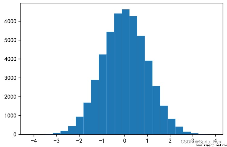
# Method 1 : adopt array Function to process a nested list into a two-dimensional array
array8 = np.array(([1, 2, 3], [4, 5, 5], [7, 8, 9]))
array8
''' array([[1, 2, 3], [4, 5, 5], [7, 8, 9]]) '''
# Method 2 : By adjusting the shape of a one-dimensional array to a two-dimensional array
temp= np.arange(1, 11)
array9 = temp.reshape((5, 2))
array9
''' array([[ 1, 2], [ 3, 4], [ 5, 6], [ 7, 8], [ 9, 10]]) '''
# Method 3 ; Create a two-dimensional array by generating random elements
array10 = np.random.randint(60, 101, (5, 3))
array10
''' array([[71, 91, 67], [95, 71, 96], [90, 91, 92], [67, 83, 74], [95, 78, 60]]) '''
# Method four : Create whole 0、 whole 1、 A two-dimensional array of specified values
array11 = np.zeros((5, 4), dtype='i8')
array11
''' array([[0, 0, 0, 0], [0, 0, 0, 0], [0, 0, 0, 0], [0, 0, 0, 0], [0, 0, 0, 0]], dtype=int64) '''
array12 = np.ones((5, 4), dtype='i8')
array12
''' array([[1, 1, 1, 1], [1, 1, 1, 1], [1, 1, 1, 1], [1, 1, 1, 1], [1, 1, 1, 1]], dtype=int64) '''
array13 = np.full((5, 4), 100)
array13
''' array([[100, 100, 100, 100], [100, 100, 100, 100], [100, 100, 100, 100], [100, 100, 100, 100], [100, 100, 100, 100]]) '''
# Method five : Create identity matrix
array14 = np.eye(5)
array14
''' array([[1., 0., 0., 0., 0.], [0., 1., 0., 0., 0.], [0., 0., 1., 0., 0.], [0., 0., 0., 1., 0.], [0., 0., 0., 0., 1.]]) '''
array10
''' array([[71, 91, 67], [95, 71, 96], [90, 91, 92], [67, 83, 74], [95, 78, 60]]) '''
# Take the specified element
array10[1][2]
# 96
array10[1, 2]
# 96
# Take some elements
array10[:3, :2]
''' array([[71, 91], [95, 71], [90, 91]]) '''
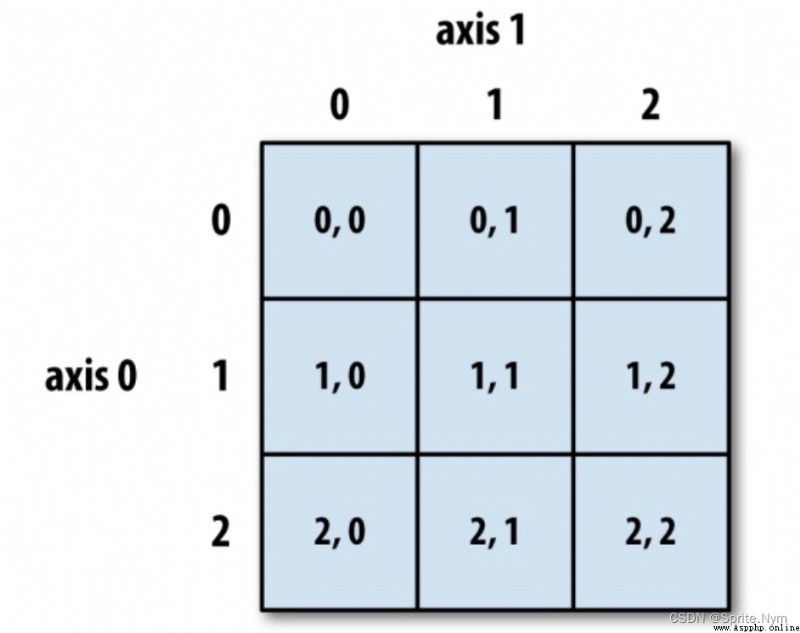
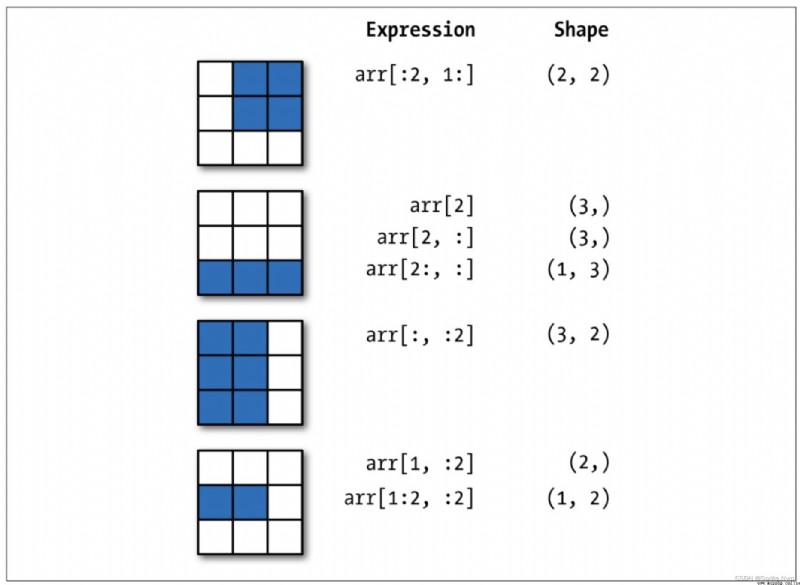
summary : In the operation of multidimensional array , Every time the index is made, the dimension is reduced , Slicing does not reduce the dimension .
# Fancy index (fancy index)
array2[[0, 1, 2, -3, -2, -1, -10]]
# array([ 1, 3, 5, 95, 97, 99, 81])
array10[[0, 1, 4], [0, 1, 2]]
# array([71, 71, 60])
# Boolean index
array1[[False, True, False, True, False]]
# array([ 2, 20], dtype=uint64)
array2[array2 > 80]
# array([81, 83, 85, 87, 89, 91, 93, 95, 97, 99])
array16 = np.arange(1, 10)
array16[array16 % 2 !=0]
# array([1, 3, 5, 7, 9])
array16[(array16 > 5) & (array16 % 2 != 0)]
# array([7, 9])
array16[(array16 > 5) | (array16 % 2 != 0)]
# array([1, 3, 5, 6, 7, 8, 9])
array16[(array16 > 5) | ~(array16 % 2 != 0)]
# array([2, 4, 6, 7, 8, 9])
array10[array10 > 80]
# array([91, 95, 96, 90, 91, 92, 83, 95])
array1 = np.random.randint(10, 50, 10)
array1
# Sum up
array1.sum
np.sum(array1)
# Averaging
array1.mean()
np.mean(array1)
# Find the median
np.median(array1)
# Find the maximum and the minimum
array1.max()
np.amax(array1)
array1.min()
np.amin(array1)
# Seeking the range ( Full range )
array1.ptp()
np.ptp(array1)
# Variance estimation
array1.var
np.var(array1)
# Find standard deviation
array1.std
np.std(array1)
# Find the cumulative sum
array1.cumsum()
np.cumsum(array1)


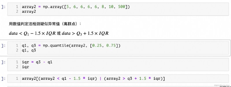
def outliers_by_iqr(t_array, lower_points = 0.25, upper_points = 0.75, whis = 1.5):
"""iqr Find outliers """
q1, q3 = np.quantile(t_array, [lower_points, upper_points])
iqr = q3 - q1
return t_array[(t_array < q1 - whis * iqr)|(t_array > q3 + whis * iqr)]
# test
array2[-1] = 15
outliers_by_iqr(array2)
# array([15])
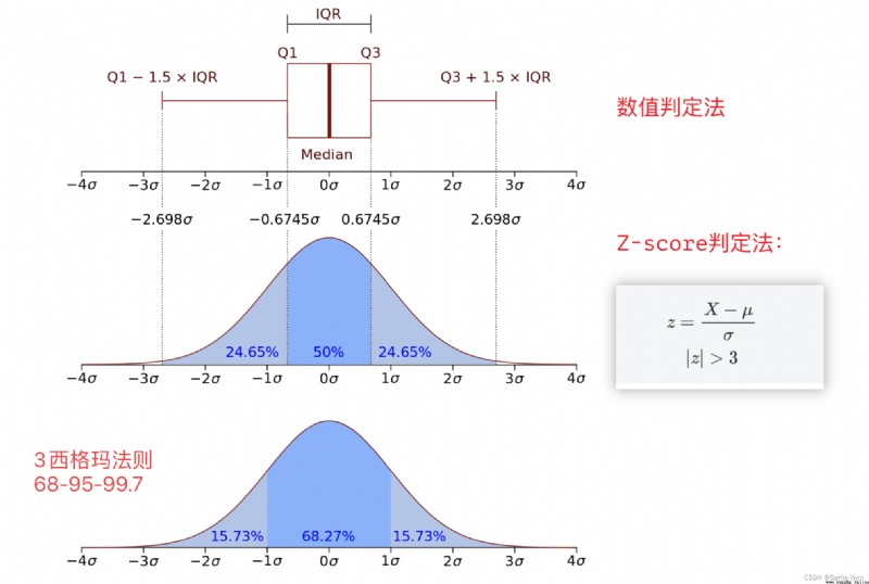
def outliers_by_zscore(array, threshold=3):
"""Z-score Decision method to detect outliers """
mu, sigma = array.mean(), array.std()
return array[np.abs((array - mu) / sigma) > threshold]
# Make the array longer , In order to make 500 It's abrupt
# repeat()( Will put the same elements together ) and tile()( Repeat in the original order )
temp = np.repeat(array2[:-1], 100)
# append() and insert() add to
temp = np.append(temp, array2[-1])
temp = np.insert(temp, 0, array2[-1])
temp
outliers_by_zscore(temp)
# array([500, 500])
Determine whether all elements in the array are True/ Determine whether the array has True The elements of .
Copy an array , And convert the elements in the array to the specified type .
array5 = array3.astype(np.float64)
array5.dtype
# dtype('float64')
Save array to file , Can pass NumPy Medium load() Function to create an array of data from a saved file .
serialize : Process objects into strings (str) Or byte string (bytes) —> Serialization / Pickles
Deserialization : Restore a string or byte string to an object —> Anti serialization
json modular :dump / dumps / load / loads —> Universal , Cross language
pickle modular :dump / dumps / load / loads —> Private agreements , Other languages cannot deserialize
# preservation
with open('array3', 'wb') as file:
array3.dump(file)
# Read
with open('array3', 'rb') as file:
array6 = np.load(file, allow_pickle=True)
array6
Fills the array with the specified elements . That is, all the elements in the array become specified elements .
Flatten a multidimensional array into a one-dimensional array
array7 = np.arange(1, 11).reshape(5, 2)
array7
''' array([[ 1, 2], [ 3, 4], [ 5, 6], [ 7, 8], [ 9, 10]]) '''
array7.flatten('C')
# array([ 1, 2, 3, 4, 5, 6, 7, 8, 9, 10])
array7.flatten('F')
# array([ 1, 3, 5, 7, 9, 2, 4, 6, 8, 10])
Return non 0 Index of elements
Round the elements in the array .
array8 = np.random.randint(1, 100, 10)
array8
# array([55, 98, 48, 98, 38, 5, 35, 36, 39, 87])
# Return the new array after sorting
np.sort(array8)
# array([ 5, 35, 36, 38, 39, 48, 55, 87, 98, 98])
array8
# array([55, 98, 48, 98, 38, 5, 35, 36, 39, 87])
# Sort in place on the original array
array8.sort()
# No return value
array8
# array([ 8, 10, 12, 27, 28, 43, 45, 57, 65, 98])
Swap axes specified by array .
# For two dimensional arrays ,transpose It is equivalent to the transpose of the matrix
array7.transpose()
''' array([[ 1, 3, 5, 7, 9], [ 2, 4, 6, 8, 10]]) '''
# swapaxes Swap the specified two axes , Order doesn't matter
array7.swapaxes(0, 1)
''' array([[ 1, 3, 5, 7, 9], [ 2, 4, 6, 8, 10]]) '''
Convert the array to Python Medium list. Do not change the original array .
array7.tolist()
# [[1, 2], [3, 4], [5, 6], [7, 8], [9, 10]]
duplicate removal .
array9 = np.array([1,1,1,1,2,2,2,3,3,3])
array9
# array([1, 1, 1, 1, 2, 2, 2, 3, 3, 3])
np.unique(array9)
# array([1, 2, 3])
array10 = np.array([[1,1,1], [2,2,2]])
array10
''' array([[1, 1, 1], [2, 2, 2]]) '''
array11 = np.array([[3,3,3,], [4,4,4,]])
array11
''' array([[3, 3, 3], [4, 4, 4]]) '''
# horizontal direction ( Along 1 Axis direction ) Stack of
np.hstack((array10, array11))
''' array([[1, 1, 1, 3, 3, 3], [2, 2, 2, 4, 4, 4]]) '''
# vertical direction ( Along 0 Axis direction ) Stack of
np.vstack((array10, array11))
''' array([[1, 1, 1], [2, 2, 2], [3, 3, 3], [4, 4, 4]]) '''
# Stack along the specified axis and increase dimension
np.stack((array10, array11), axis=0)
''' array([[[1, 1, 1], [2, 2, 2]], [[3, 3, 3], [4, 4, 4]]]) '''
np.stack((array10, array11), axis=1)
''' array([[[1, 1, 1], [3, 3, 3]], [[2, 2, 2], [4, 4, 4]]]) '''
array12 = np.concatenate((array10, array11), axis=0)
array12
''' array([[1, 1, 1], [2, 2, 2], [3, 3, 3], [4, 4, 4]]) '''
array13 = np.concatenate((array10, array11), axis=1)
array13
''' array([[1, 1, 1, 3, 3, 3], [2, 2, 2, 4, 4, 4]]) '''
# vertical direction ( Along 0 Axis direction ) The split
np.vsplit(array12, 2)
''' [array([[1, 1, 1], [2, 2, 2]]), array([[3, 3, 3], [4, 4, 4]])] '''
np.vsplit(array12, 4)
''' [array([[1, 1, 1]]), array([[2, 2, 2]]), array([[3, 3, 3]]), array([[4, 4, 4]])] '''
# horizontal direction ( Along 1 Axis direction ) The split
np.hsplit(array12, 3)
''' [array([[1], [2], [3], [4]]), array([[1], [2], [3], [4]]), array([[1], [2], [3], [4]])] '''
# Split along the specified axis
np.split(array13, 2)
''' [array([[1, 1, 1, 3, 3, 3]]), array([[2, 2, 2, 4, 4, 4]])] '''
np.split(array13, 3, axis=1)
''' [array([[1, 1], [2, 2]]), array([[1, 3], [2, 4]]), array([[3, 3], [4, 4]])] '''
# Extract elements from the array according to the specified conditions ( Similar to Boolean index )
np.extract(array14 <= 50, array14)
# array([19, 23, 50])
array14[array14 <= 50]
# array([19, 23, 50])
# Process the elements in the array according to the condition list to get a new array ( Multiple conditions )
np.select([array14 % 2 == 0, array14 % 2 != 0], [array14 / 2, array14 ** 2])
# array([ 361., 9025., 38., 529., 25.])
# Get a new array according to the elements in the condition array ( Single condition )
np.where(array14 % 2 == 0, array14, 0)
# array([ 0, 0, 76, 0, 50])
From left to right , Cycle filling from top to bottom
array15 = np.arange(1, 10).reshape((3, 3))
array15
''' array([[1, 2, 3], [4, 5, 6], [7, 8, 9]]) '''
# Size the array
np.resize(array15, (4, 4))
''' array([[1, 2, 3, 4], [5, 6, 7, 8], [9, 1, 2, 3], [4, 5, 6, 7]]) '''
# Replace the element with the specified index in the array
np.put(array15, 5, 100)
array15
''' array([[ 1, 2, 3], [ 4, 5, 100], [ 7, 8, 9]]) '''
np.put(array15, [1, 2], 100)
array15
''' array([[ 1, 100, 100], [ 4, 5, 100], [ 7, 8, 9]]) '''
# Replace the elements in the array that meet the conditions
np.place(array15, array15 == 100, [2, 3])
array15
''' array([[1, 2, 3], [4, 5, 2], [7, 8, 9]]) '''
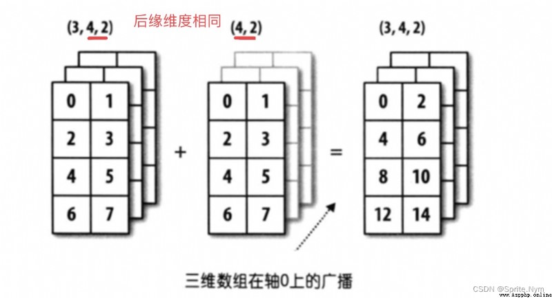
Prerequisite ( One of these must be met ):
The trailing dimension of two arrays (shape Attributes look back and forward ) identical .
The trailing edge dimensions of the two arrays are different , But one of the dimensions is 1.
The broadcast mechanism is satisfied to follow the missing axis or along the dimension 1 The axis broadcasts itself , Eventually the shape becomes uniform .
# Meet the conditions 1:
array16 = np.arange(1, 16).reshape(5, 3)
array17 = np.array([[1, 1, 1]])
array16 + array17
''' array([[ 2, 3, 4], [ 5, 6, 7], [ 8, 9, 10], [11, 12, 13], [14, 15, 16]]) '''
# Still meet the conditions 1:
array18 = np.random.randint(1, 18, (3, 4, 2))
array18
''' array([[[ 2, 11], [17, 16], [ 2, 6], [ 3, 13]], [[ 6, 17], [15, 4], [ 2, 2], [ 9, 6]], [[ 8, 4], [ 5, 9], [15, 11], [ 6, 17]]]) '''
array19 = np.random.randint(1, 10, (4, 2))
array19
''' array([[7, 5], [1, 7], [2, 7], [6, 5]]) '''


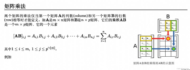
A ⋅ B = ∑ a i b i A \cdot B = \sum a_ib_i \\ A⋅B=∑aibi
A ⋅ B = ∣ A ∣ ∣ B ∣ c o s θ A \cdot B = |A||B|cos\theta A⋅B=∣A∣∣B∣cosθ
Calculated as scalar
# Find the dot product
a = np.array([1, 2, 3])
b = np.array([2, 4, 6])
np.dot(a, b)
# 28, namely 1 * 2 + 2 * 4 + 3 * 6 = 28
# seek a The mold
# linear algebra
np.linalg.norm(a)
# seek b The mold
np.linalg.norm(b)
# seek a,b Cosine of the included angle , And then you get a,b The relevance of
np.dot(a, b) / np.linalg.norm(a) / np.linalg.norm(b)
# 1.0
# Create a matrix
m1 = np.matrix('1 2; 3 4')
m1
''' matrix([[1, 2], [3, 4]]) '''
type(m1)
# numpy.matrix
# Get the corresponding array object
m1.A
''' array([[1, 2], [3, 4]]) '''
# Get the corresponding flattened array object
m1.A1
''' array([1, 2, 3, 4]) '''
# Get the transposed matrix
m1.T
''' matrix([[1, 3], [2, 4]]) '''
m1.swapaxes(0, 1)
m1.transpose()
# Empathy
# Get the inverse matrix
m1.I
''' matrix([[-2. , 1. ], [ 1.5, -0.5]]) '''
A ⋅ A − 1 = I A \cdot A^{-1} = I A⋅A−1=I
m2 = np.matrix('1 0 2; -1 3 1')
m2
''' matrix([[ 1, 0, 2], [-1, 3, 1]]) '''
m3 = np.mat([[3, 1], [2, 1], [1, 0]])
m3
''' matrix([[3, 1], [2, 1], [1, 0]]) '''
m2 * m3
''' matrix([[5, 1], [4, 2]]) '''
# Create from nested lists or 2D arrays matrix object
m4 = np.asmatrix(np.arange(1, 10).reshape((3, 3)))
m4
''' matrix([[1, 2, 3], [4, 5, 6], [7, 8, 9]]) '''
# determinent
# Calculate the value of the matrix
np.linalg.det(m4)
# Calculate the rank of the matrix
np.linalg.matrix_rank(m4)
array2 = m2.A
array2
''' array([[ 1, 0, 2], [-1, 3, 1]]) '''
array3 = m3.A
array3
''' array([[3, 1], [2, 1], [1, 0]]) '''
# Matrix multiplication of array objects
array2 @ array3
''' array([[5, 1], [4, 2]]) '''
# Inverse matrix
array1 = m1.A
np.linalg.inv(array1)
''' array([[-2. , 1. ], [ 1.5, -0.5]]) '''
{ x 1 + 2 x 2 + x 3 = 8 3 x 1 + 7 x 2 + 2 x 3 = 23 2 x 1 + 2 x 2 + x 3 = 9 \begin{cases} x_1 + 2x_2 + x_3 = 8 \\ 3x_1 + 7x_2 + 2x_3 = 23 \\ 2x_1 + 2x_2 + x_3 = 9 \end{cases} ⎩⎪⎨⎪⎧x1+2x2+x3=83x1+7x2+2x3=232x1+2x2+x3=9
A ⋅ x = b A \cdot x = b A⋅x=b
A = np.array([[1, 2, 1], [3, 7, 2], [2, 2, 1]])
b = np.array([8, 23, 9]).reshape(-1, 1)
C = np.hstack((A, b))
C
''' array([[ 1, 2, 1, 9], [ 3, 7, 2, 23], [ 2, 2, 1, 9]]) '''
np.linalg.matrix_rank(A)
# 3
np.linalg.matrix_rank(C)
# 3
A ⋅ x = b A − 1 ⋅ A ⋅ x = A − 1 ⋅ b I ⋅ x = A − 1 ⋅ b x = A − 1 ⋅ b A \cdot x = b \\ A^{-1} \cdot A \cdot x = A^{-1} \cdot b \\ I \cdot x = A^{-1} \cdot b \\ x = A^{-1} \cdot b \\ A⋅x=bA−1⋅A⋅x=A−1⋅bI⋅x=A−1⋅bx=A−1⋅b
# Use the above formula to solve linear equations
np.linalg.inv(A) @ b
''' array([[1.], [2.], [3.]]) '''
# Solve a system of linear equations
np.linalg.solve(A, b)
''' array([[1.], [2.], [3.]]) '''
# Download the machine learning module
pip install scikit-learn
import warnings
warnings.filterwarnings('ignore')
from sklearn.datasets import load_boston
# Load Boston house price data set
datasets = load_boston()
# see datasets attribute
dir(datasets)
# ['DESCR', 'data', 'data_module', 'feature_names', 'filename', 'target']
# Print content description
print(datasets.DESCR)
# Too much content to show
# Print influencing factor data
datasets.data
# Too much content to show
# View data type
type(datasets.data)
# numpy.ndarray
# see shape
datasets.data.shape
# (506, 13)
# View the influencing factor name
datasets.feature_names
''' array(['CRIM', 'ZN', 'INDUS', 'CHAS', 'NOX', 'RM', 'AGE', 'DIS', 'RAD', 'TAX', 'PTRATIO', 'B', 'LSTAT'], dtype='<U7') '''
# Get house price data
y = datasets.target
y.shape
# (506,)
# Get crime rate data
x1 = datasets.data[:, 0]
x1.shape
# (506,)
# Calculate the correlation coefficient between crime rate and house price
np.corrcoef(x1, y)
''' array([[ 1. , -0.38830461], [-0.38830461, 1. ]]) '''
# Access to data on low-income groups
x2 = datasets.data[:, -1]
x2.shape
# (506,)
# Calculate the correlation coefficient between low-income groups and house prices
np.corrcoef(x2, y)
''' array([[ 1. , -0.73766273], [-0.73766273, 1. ]]) '''
# The following same example omits
# Draw a scatter diagram
plt.scatter(x1, y)
plt.scatter(x2, y)
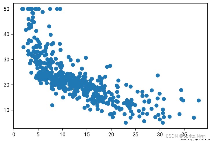
# obtain x: Average room count data ,y: House price data
x = datasets.data[:, 5]
y = datasets.target
# Store historical data in a dictionary
history_data = {
}
delta = 0
for room, price in zip(x, y):
if room not in history_data:
history_data[room] = price
else:
delta += 0.000001
history_data[room + delta] = price
len(history_data)
# 506
import heapq
def predicate_by_knn(room_num, k=5):
# Find the nearest... To the target data k Historical data
nearest_neighbors = heapq.nsmallest(k, history_data, key=lambda x:(x-room_num) ** 2)
# Calculate the average of the values corresponding to these keys in the historical data
return round(np.mean([history_data[key] for key in nearest_neighbors]), 2)
# Call the function to try
predicate_by_knn(6.125)
# 22.12
predicate_by_knn(5.525)
# 13.32
def get_loss(x, y, a, b):
""" Loss function """
return np.mean((a * x + b - y) ** 2)
# Start Monte Carlo simulation , If the error is lower, record it
min_loss = np.inf
best_a, best_b = None, None
for _ in range(10000):
a, b = np.random.random(2) * 200 - 100
curr_loss = get_loss(x, y, a, b)
if curr_loss < min_loss:
min_loss = curr_loss
best_a, best_b = a, b
print(a, b, min_loss)
print(best_a, best_b)
y_hat = best_a * x + best_b
# Draw a picture to see
plt.scatter(x, y)
plt.plot(x, y_hat, color='red', linewidth=8)
# Define the function to calculate the predicted value according to the fitting curve
def predicate_by_regression(room_num):
return round(best_a * room_num + best_b, 2)
# Call the function to try
predicate_by_regression(5.525)
# 15
# seek a Partial derivative of
def partial_a(x, y, a, b):
return 2 * np.mean((y - a * x - b) * (-x))
# seek b Partial derivative of
def partial_b(x, y, a, b):
return 2 * np.mean(-y + a * x + b)
# Use gradient descent algorithm to find a, b
a, b = 50, -50
delta = 0.013
for _ in range(1000):
a = a - partial_a(x, y, a, b) * delta
b = b - partial_b(x, y, a, b) * delta
print(get_loss(x, y, a, b))
print(best_a, best_b)
param1 = np.vstack((x, np.ones(x.size))).T
param1
param2 = y.reshape((-1, 1))
param2
# least square - Least square solution
results = np.linalg.lstsq(param1, param2)
results
''' (array([[ 9.10210898], [-34.67062078]]), array([22061.87919621]), 2, array([143.99484122, 2.46656609])) '''
a, b = results[0].flatten()
a, b
# (9.102108981180313, -34.67062077643857)
y_hat = a * x + b
plt.scatter(x, y)
plt.plot(x, y_hat, color='red', linewidth=8)
# establish Series object
ser1 = pd.Series(data=[320, 180, 250, 220], index=[f'{
x} quarter ' for x in '1234'])
ser1
''' 1 quarter 320 2 quarter 180 3 quarter 250 4 quarter 220 dtype: int64 '''
# Create... From a dictionary series object
ser2 = pd.Series(data={
' First quarter ': 320, ' The two quarter ': 180, ' third quater ': 250, ' In the fourth quarter ': 220})
ser2
''' First quarter 320 The two quarter 180 third quater 250 In the fourth quarter 220 dtype: int64 '''
# General index
ser1['1 quarter ']
# 320
ser2. First quarter
# 320 ( This query method cannot be changed to 1 quarter , Because the number can't start )
# Fancy index
ser1[['1 quarter ', '3 quarter ']]
''' 1 quarter 320 3 quarter 250 dtype: int64 '''
# Boolean index
ser1[ser1 >= 200]
''' 1 quarter 320 3 quarter 250 4 quarter 220 dtype: int64 '''
ser1[1:3]
''' 2 quarter 180 3 quarter 250 dtype: int64 '''
# Slice with your own index name. You can get it at both ends
ser1['2 quarter ': '3 quarter ']
''' 2 quarter 180 3 quarter 250 dtype: int64 '''
# Get index
ser2.index
# Index([' First quarter ', ' The two quarter ', ' third quater ', ' In the fourth quarter '], dtype='object')
# Get the value of the index
ser2.index.values
# array([' First quarter ', ' The two quarter ', ' third quater ', ' In the fourth quarter '], dtype=object)
# get data
ser2.values
# array([320, 180, 250, 220], dtype=int64)
# Element number
ser2.size
# 4
# Is the element unique
ser2.is_unique
# True
# Is there a null value
ser2.hasnans
# False
ser2[' The two quarter '] = np.nan
ser2
''' First quarter 320.0 The two quarter NaN third quater 250.0 In the fourth quarter 220.0 dtype: float64 '''
ser2.hasnans
# True
ser2[' The two quarter '] = 280
ser2
# 280
# Whether the data is monotonically increasing
ser2.is_monotonic_increasing
# False
# Whether the data is monotonically decreasing
ser2.is_monotonic_decreasing
# True
# Get descriptive statistics - Concentration trend
# Sum up
print(ser2.sum())
# Averaging
print(ser2.mean())
# Median
print(ser2.median())
''' 1070.0 267.5 265.0 '''
# The number of
print(ser2.mode())
''' 0 220.0 1 250.0 2 280.0 3 320.0 dtype: float64 '''
# Get descriptive statistics - Discrete trends
# Maximum and minimum
print(ser2.max())
print(ser2.min())
# Variance and standard deviation
print(ser2.var())
print(ser2.std())
print(np.var(ser2))
print(np.std(ser2))
# The upper and lower quartiles
print(ser2.quantile(0.25))
print(ser2.quantile(0.75))
print(np.quantile(ser2, (0.25, 0.5, 0.75)))
''' 320 220 1825.0 42.720018726587654 1368.75 36.99662146737185 242.5 290.0 [242.5 265. 290. ] '''
# Get all descriptive statistics directly
ser2.describe()
''' count 4.000000 mean 267.500000 std 42.720019 min 220.000000 25% 242.500000 50% 265.000000 75% 290.000000 max 320.000000 dtype: float64 '''
ser3 = pd.Series(['apple', 'banana', 'apple', 'pitaya', 'apple', 'pitaya', 'durian'])
ser3
''' 0 apple 1 banana 2 apple 3 pitaya 4 apple 5 pitaya 6 durian dtype: object '''
# duplicate removal ---> ndarray
ser3.unique()
# array(['apple', 'banana', 'pitaya', 'durian'], dtype=object)
# The number of non repeating elements
ser3.nunique()
# 4
# The frequency of element repetition ( In descending order of frequency )
ser3.value_counts()
''' apple 3 pitaya 2 banana 1 durian 1 dtype: int64 '''
# Judge whether the elements are repeated
ser3.duplicated()
''' 0 False 1 False 2 True 3 False 4 True 5 True 6 False dtype: bool '''
# Boolean index de duplication
ser3[~ser3.duplicated()]
''' 0 apple 1 banana 3 pitaya 6 durian dtype: object '''
# duplicate removal ---> Series
ser3.drop_duplicates()
''' 0 apple 1 banana 3 pitaya 6 durian dtype: object '''
# keep - The repeating element retains the first or last item , The default value is first
ser3.drop_duplicates(keep='last')
''' 1 banana 4 apple 5 pitaya 6 durian dtype: object '''
# inplace - Whether to operate locally
# True ---> Local operation , Do not return new objects ---> None
# False( The default value is )---> Return the new object after the operation ---> Series
ser3.drop_duplicates(keep=False, inplace=True)
ser3
''' 1 banana 6 durian dtype: object '''
# Judge null
ser4.isnull()
''' 0 False 1 False 2 True 3 False 4 True dtype: bool '''
# Judge non null value
ser4.notnull()
''' 0 True 1 True 2 False 3 True 4 False dtype: bool '''
# Filter non null values by Boolean index
ser4[ser4.notnull()]
''' 0 10.0 1 20.0 3 30.0 dtype: float64 '''
# Delete the specified data
ser4.drop(index=2)
''' 0 10.0 1 20.0 3 30.0 4 NaN dtype: float64 '''
ser4.drop(index=[2, 4])
''' 0 10.0 1 20.0 3 30.0 dtype: float64 '''
# Delete null (inplace=True, Delete in place )
ser4.dropna()
''' 0 10.0 1 20.0 3 30.0 dtype: float64 '''
# Fill in empty values
ser4.fillna(50)
''' 0 10.0 1 20.0 2 50.0 3 30.0 4 50.0 dtype: float64 '''
ser4.fillna(method='ffill')
''' 0 10.0 1 20.0 2 20.0 3 30.0 4 30.0 dtype: float64 '''
ser4.fillna(method='bfill')
''' 0 10.0 1 20.0 2 30.0 3 30.0 4 NaN dtype: float64 '''
# Fill both front and back once
ser4.fillna(method='ffill').fillna(method='bfill')
# Sort the index
# ascending ---> Ascending or descending ---> The default value is True, Represents ascending order
ser1.sort_index(ascending=False)
''' 4 quarter 220 3 quarter 250 2 quarter 180 1 quarter 320 dtype: int64 '''
# Sort values
ser1.sort_values(ascending=False)
''' 1 quarter 320 3 quarter 250 4 quarter 220 2 quarter 180 dtype: int64 '''
# Top-N
ser1.nlargest(3)
''' 1 quarter 320 3 quarter 250 4 quarter 220 dtype: int64 '''
ser1.nsmallest(2)
''' 2 quarter 180 4 quarter 220 dtype: int64 '''
# example 1:format Batch process strings
ser5 = pd.Series(['cat', 'dog', np.nan, 'rabbit'])
ser5
''' 0 cat 1 dog 2 NaN 3 rabbit dtype: object '''
ser5.map('I am a {}'.format, na_action='ignore')
''' 0 I am a cat 1 I am a dog 2 NaN 3 I am a rabbit dtype: object '''
# example 2: Batch processing of data
ser6 = pd.Series(np.random.randint(30, 80, 10))
ser6
''' 0 62 1 67 2 65 3 64 4 64 5 31 6 76 7 42 8 54 9 45 dtype: int32 '''
# following 3 Either way
def upgrade(score):
return score ** 0.5 * 10
# np.round(ser6.map(upgrade), 0)
# np.round(ser6.map(lambda x: x ** .5 * 10), 0)
np.round(ser6.apply(lambda x: x ** .5 * 10), 0)
''' 0 79.0 1 82.0 2 81.0 3 80.0 4 80.0 5 56.0 6 87.0 7 65.0 8 73.0 9 67.0 dtype: float64 '''
Linear normalization ( Standardization ):
X i ′ = X i − X m i n X m a x − X m i n X_i' = \frac {X_{i} - X_{min}} {X_{max} - X_{min}} Xi′=Xmax−XminXi−Xmin
Zero mean normalization ( Centralization ):
X i ′ = X i − μ σ X_i' = \frac {X_{i} - \mu} {\sigma} Xi′=σXi−μ
# example 3: Normalize the data
ser7 = pd.Series(data=np.random.randint(1, 10000, 10))
ser7
''' 0 9359 1 1222 2 2843 3 985 4 2478 5 3935 6 6838 7 1999 8 5907 9 9064 dtype: int32 '''
# Linear normalization
x_min = ser7.min()
x_max = ser7.max()
ser7.map(lambda x: (x - x_min) / (x_max - x_min))
''' 0 1.000000 1 0.028302 2 0.221877 3 0.000000 4 0.178290 5 0.352281 6 0.698949 7 0.121089 8 0.587772 9 0.964772 dtype: float64 '''
# Zero mean normalization
miu = ser7.mean()
sigma = ser7.std()
ser7.map(lambda x: (x - miu) / sigma)
''' 0 1.646880 1 -1.090183 2 -0.544923 3 -1.169903 4 -0.667699 5 -0.177605 6 0.798885 7 -0.828822 8 0.485722 9 1.547650 dtype: float64 '''
ser7 = pd.Series(
data = np.random.randint(150, 550, 8),
index = [f'{
x} quarter ' for x in '11213434']
)
ser7
''' 1 quarter 322 1 quarter 440 2 quarter 348 1 quarter 256 3 quarter 242 4 quarter 483 3 quarter 401 4 quarter 448 dtype: int32 '''
# Draw a pie chart based on quarterly summary data
# level = 0 According to the said 0 Level index grouping
temp = ser7.groupby(level=0).sum()
temp
''' 1 quarter 1018 2 quarter 348 3 quarter 643 4 quarter 931 dtype: int32 '''
# Draw a histogram
temp.plot(kind='bar', color=['#a3f3b4', '#D8F781', 'blue', 'pink'])
plt.xticks(rotation=0)
plt.grid(True, alpha=0.5, axis='y', linestyle=':')
plt.show()
# Draw the pie chart
temp.plot(kind='pie', autopct='%.2f%%', wedgeprops={

'edgecolor': 'w',
'width': 0.4,
}, pctdistance=0.8)
# Change y Axis labels
plt.ylabel('')
plt.show()
stuids = np.arange(1001, 1006)
courses = [' Chinese language and literature ', ' mathematics ', ' English ']
scores = np.random.randint(60, 101, (5, 3))
# Method 1: Create by 2D array or nesting DataFrame object
df1 = pd.DataFrame(data = scores, columns = courses, index = stuids)
df1
# Method 2: Create... From a dictionary DataFrame object
scores = {

' Chinese language and literature ': [62, 72, 93, 88, 93],
' mathematics ': [95, 65, 86, 66, 87],
' English ': [66, 75, 82, 69, 82]
}
df2 = pd.DataFrame(data = scores, index = stuids)
df2
# Read CSV File creation DataFrame object
df4 = pd.read_csv(
'datas/2018 Beijing points settlement data in .csv',
index_col='id', # Specify index columns
sep='#', # Specify the separator
quotechar='`', # The characters of the package contents
usecols=['id', 'name', 'score'], # Which columns to read
nrows=10, # Number of rows read
skiprows=np.arange(1, 11) # Number of lines skipped
# skiprows=lambda rn: rn > 0 and random.random() < 0.9 # Number of randomly skipped rows
)
df4
# Read CSV File and create an iterator object
df5_iter = pd.read_csv(
'datas/bilibili.csv',
encoding='gbk',
chunksize=10, # 10 A content 1 box
iterator=True # Create an iterator object
)
df5_iter
# Get... Through iterators DataFrame object
next(df5_iter)
df6 = pd.read_excel('datas/ Data of national tourist attractions .xlsx')
df6
# Omit the result presentation
df7 = pd.read_excel(
'datas/2020 Annual sales figures .xlsx',
sheet_name='data', # Name of the table to read
header=0, # Specify header position
nrows=500,
skiprows=np.arange(1, 502)
)
df7
# Omit the result presentation
df8 = pd.read_excel(
'datas/ Figures of the Three Kingdoms .xlsx',
sheet_name=' All character data ',
header=0,
usecols=np.arange(0, 10)
)
df8
# Omit the result presentation
# establish conn object
import pymysql
conn = pymysql.connect(host='47.104.31.138', port=3306,
user='guest', password='Guest.618',
database='hrs', charset='utf8mb4')
conn
# <pymysql.connections.Connection at 0x1c469df74f0>
# Or create engine object
from sqlalchemy import create_engine
engine = create_engine('mysql+pymysql://guest:[email protected]/hrs')
engine
# from engine Object or conn Object to extract data
dept_df = pd.read_sql('select dno, dname, dloc from tb_dept', conn)
dept_df
# Omit the result presentation
emp_df = pd.read_sql('select eno, ename, job, sal, comm, dno from tb_emp', engine)
emp_df
# Omit the result presentation
from sqlalchemy import create_engine
engine = create_engine('mysql+pymysql://guest:[email protected]:3306/hrs')
engine
# Get department table
dept_df = pd.read_sql('select dno, dname, dloc from tb_dept', engine)
dept_df
# Get employee table
emp_df = pd.read_sql('select eno, ename, job, sal, comm, dno from tb_emp', engine)
emp_df
# use DataFrame The method of inner connection
emp_df.merge(dept_df, how='inner', on='dno')
# After changing the column name , The column names of the two tables are no longer equal
dept_df.rename(columns={
'dno': 'deptno'}, inplace=True)
# use left_on and right_on Set associated table conditions
temp_df = emp_df.merge(dept_df, how='inner', left_on='dno', right_on='deptno')
temp_df
# You can also use functions to join tables
temp_df = pd.merge(emp_df, dept_df, how='inner',
left_on='dno', right_on='deptno')
temp_df
# At this time, the same columns used in the join table will not be automatically merged , Can be deleted manually
temp_df.drop(columns=['deptno', 'job'], inplace=True)
# take deptno Change column to index column
dept_df = dept_df.set_index('deptno')
# When the join condition is the index column, write right_index=True
pd.merge(emp_df, dept_df, how='inner', left_on='dno', right_index=True)
import os
# ignore_index=True It means that the original number is ignored and renumbered
df1 = pd.concat([pd.read_csv(f'datas/jobs/{
i}') for i in os.listdir('datas/jobs')],
ignore_index=True)
df1.drop(columns=['uri', 'city'], inplace=True)
df1
# 1. Operation column
# Get the specified column
df1['site']
# Calculate the number of companies without repetition
df1['company_name'].nunique()
# duplicate removal
df1['company_name'].drop_duplicates()
# Fancy indexes get multiple columns at the same time
df1[['company_name', 'site', 'edu']]
# Boolean index
df1[df1['edu']==' Undergraduate ']
# Get multiple rows by index column and column name at the same time
df1.loc[[4, 7, 1]]
# Slice multiple rows according to the built-in index
df1.iloc[1:5]
# Slice multiple rows by index column
df1.loc[1:5]
# 2. Action cell
# Lock cells by index column and column name
df1.at[7, 'company_name']
# Lock cells by number
df1.iat[7, 0]
# Change cell
df1.iat[7, 0] = ' A capitalist of Sichuan University '
Be careful :iloc and loc、iat and at, No addition i Means to search by row name and column name , added i Means to search by index number .
# Judge whether it is a null value
emp_df.isnull()
# Determine whether it is a non null value
emp_df.notnull()
# Delete rows with null values ( That is, along 0 Axis deletion )
emp_df.dropna()
# Delete columns with null values ( That is, along 1 Axis deletion )
emp_df.dropna(axis=1)
# Fill in the null value of the specified column ( Since each column has different requirements for handling null values , So, one column at a time )
emp_df['comm'] = emp_df['comm'].fillna(0).astype(np.int64)
emp_df
# Judgment repeats
emp_df.duplicated('job')
# duplicate removal
emp_df.drop_duplicates('job', keep='first')
# obtain DataFrame Information about the object
ytb.info()
# obtain DataFrame The front of the object 10 That's ok
ytb.head(10)
# obtain DataFrame After the object 10 That's ok
ytb.tail(10)
Case study :
# Do not limit the maximum number of columns displayed
pd.set_option('display.max_column', None)
# Read Kobe's shooting data sheet
kobe = pd.read_csv('datas/Kobe_data.csv', index_col='shot_id')
kobe
# Check the information
kobe.info()
# Count the number of matches
kobe['game_id'].nunique()
# Count which team you have played against the most
kobe.drop_duplicates('game_id', inplace=True)
ser = kobe['opponent'].value_counts()
ser.index[0]
# Delete by index
kobe.drop(index=kobe[kobe['opponent']=='BKN'].index)
# Replace the specified cell with ( First limit to the target column , Lest other places be inadvertently replaced )
kobe['opponent'] = kobe['opponent'].replace(['SEA', 'BKN'], ['OKC', 'NJN'])
# Regular expression substitution
kobe = kobe.replace('BKN|SEA', '---', regex=True)
# String to time date
kobe['game_date'] = pd.to_datetime(kobe['game_date'])
# Get the year in the time date 、 quarter 、 month
kobe['year'] = kobe['game_date'].dt.year
kobe['quarter'] = kobe['game_date'].dt.quarter
kobe['month'] = kobe['game_date'].dt.month
# .str Get the string corresponding to the data series , Readjust the string method
kobe['opponent'] = kobe['opponent'].str.lower()
kobe
# Screening job_type by python Or the position of data analysis
jobs_df.query('job_type == "python" or job_type == " Data analysis "')
# Screening job_name contain python Or data analysis
jobs_df = jobs_df[jobs_df['job_name'].str.lower().str.contains('python') |
jobs_df['job_name'].str.contains(' Data analysis ')]
# Use regular expression capture group to extract data
temp_df = jobs_df['salary'].str.extract(r'(\d+)[Kk]?-(\d+)[Kk]?')
# adopt applymap Methods will DataFrame Each element of is processed into int type
temp_df = temp_df.applymap(int)
temp_df.info()
# Along 1 Average the axis
jobs_df['salary'] = temp_df.mean(axis=1)
jobs_df
# Split site Column
temp_df = jobs_df['site'].str.split(r'\s', expand=True, regex=True)
temp_df.rename(columns={
0: 'city', 1: 'district', 2: 'street'}, inplace=True)
temp_df
# Add a column directly
jobs_df[temp_df.columns] = temp_df
jobs_df
# Delete the specified column
jobs_df.drop(columns='site', inplace=True)
jobs_df
# Through intra index join
jobs_df.merge(temp_df, how='inner', left_index=True, right_index=True)
Be careful :apply and map yes Series Methods , and applymap yes DataFrame Methods .
# Reorder indexes
jobs_df.reindex(columns=['company_name', 'city', 'district', 'street', 'salary', 'year', 'edu', 'job_name', 'job_type'])
# Adjust the order of columns with fancy indexes
jobs_df[['company_name', 'city', 'district', 'street', 'salary', 'year', 'edu', 'job_name', 'job_type']]
# Get the target row by Boolean index and delete
jobs_df.drop(index=jobs_df[(jobs_df['edu'] == ' high school ') | (jobs_df['edu'] == ' secondary specialized school ')].index,
inplace=True)
jobs_df
jobs_df['min_exp'] = jobs_df['year'].replace(['1 Within years ', ' Experience is unlimited ', ' Fresh graduates '],
['0-1 year ', '0 year ', '0 year ']).str.extract(r'(\d+)')
jobs_df
# Let's first look at the data distribution
luohu_df['score'].describe()
# Separate boxes
score_seg = pd.cut(luohu_df['score'], bins=np.arange(90, 130, 5), right=False)
score_seg
# Add back the data after sorting
luohu_df.insert(4, 'score_seg', score_seg)
luohu_df
# Count the quantity of each box
ser2 = luohu_df['score_seg'].value_counts()
ser2
# Draw a histogram
ser2.plot(kind='bar')
for i, index in enumerate(ser2.index):
# The first parameter is x Axis position , The second is y Axis position , The third is the displayed string , The fourth is center alignment
plt.text(i, ser2[index] + 20, ser2[index], ha='center')
# x The shaft scale rotates counterclockwise 30 degree
plt.xticks(rotation=30)
# Create dummy variable matrix
temp_df = pd.get_dummies(persons_df[' occupation '])
''' Doctor Teachers' Painter The programmer 0 1 0 0 0 1 1 0 0 0 2 0 0 0 1 3 0 0 1 0 4 0 1 0 0 '''
# Write back to the original table
persons_df[temp_df.columns] = temp_df
persons_df
# Delete the original occupation column
persons_df.drop(columns=' occupation ', inplace=True)
persons_df
# use apply Mapping functions process ordered variables into numeric values
def edu_to_value(sc):
results = {
' high school ': 1, ' junior college ': 3, ' Undergraduate ': 5, ' Graduate student ': 10}
return results.get(sc, 0)
persons_df[' Education '] = persons_df[' Education '].apply(edu_to_value)
persons_df
# Import data
sales_df = pd.read_excel('datas/2020 Annual sales figures .xlsx', sheet_name='data')
sales_df
# Check the information
sales_df.info()
# Calculate sales
sales_df[' sales '] = sales_df[' sales volumes '] * sales_df[' The price is ']
sales_df
# Calculate the average value of sales per order
sales_df[' sales '].sum() / sales_df[' Sales order '].nunique()
# Get descriptive statistics
sales_df[' sales volumes '].describe()
# take DataFrame Objects are in descending order by sales ( If you want to sort by multiple keywords, use a list ,ascending Followed by a list )
sales_df.sort_values(by=[' sales '], ascending=False)
# Take the top one with the largest sales 10 Data
sales_df.nlargest(10, ' sales ')
# Take the top one with the smallest sales 5 Data
sales_df.nsmallest(5, ' sales ')
# 1. Statistics 2020 Monthly sales amount
# Add the writing of the month column
sales_df[' month '] = sales_df[' Sales date '].dt.month
sales_df.groupby(' month ')[[' sales ']].sum()
# Do not add the month column ( The column names of the resulting tables are still the same ‘ Sales date ’)
sales_df.groupby(sales_df[' Sales date '].dt.month)[[' sales ']].sum()
# 2. Statistics on the proportion of sales of various brands
total_sales = sales_df[' sales '].sum()
ser = sales_df.groupby(' brand ')[' sales '].sum()
ser / total_sales
# Draw a pie chart ( Don't count the percentage yourself , Will automatically calculate )
ser.plot(kind='pie', autopct='%.1f%%', pctdistance=1.3)
# 3. Count the monthly sales of each region
# Method 1: own groupby polymerization
# Multi level index ( In this case, the sales region and month are used as index columns )
temp_df = sales_df.groupby([' Sales area ', ' month '])[[' sales ']].sum()
temp_df
# Reset index ( At this point, the sales region and month become common columns )
temp_df = temp_df.reset_index()
temp_df
# perspective ( Specify who is the index 、 Who is column 、 Who is worth )
temp_df2 = temp_df.pivot(index=' Sales area ', columns=' month ', values=' sales ').fillna(0).applymap(int)
temp_df2
# Method 2: One step in place
# Generate pivot table ---> according to A Statistics B
sales_df.pivot_table(
index=' Sales area ',
columns=' month ',
values=' sales ',
aggfunc=np.sum, # You can use multiple aggregate functions at the same time , Transfer list
fill_value=0,
margins=True, # Add summary row 、 Column
margins_name=' A total of ' # Remit to the head office 、 Column name
).applymap(int)
# 4. Count the brand sales of each channel
pd.pivot_table(
sales_df, index=' Distribution channel ', columns=' brand ', values=' sales volumes ',
aggfunc='sum', margins=True, margins_name=' A total of '
)
# 5. Calculate the monthly sales volume proportion of different price ranges
sales_df[' The price is '].describe()
# Method 1: Conditional column
# Define the condition of the condition column
def make_tag(price):
if price < 200:
return ' Low-end '
return ' Middle end ' if price < 470 else ' High-end '
# Create condition column
sales_df[' Price '] = sales_df[' The price is '].apply(make_tag)
sales_df
# PivotTable
temp_df = pd.pivot_table(sales_df, index=' Price ', columns=' month ', values=' sales volumes ', aggfunc='sum')
temp_df
# The order of changing careers
temp_df = temp_df.reindex(index=[' Low-end ', ' Middle end ', ' High-end '])
temp_df
# Method 2: Separate boxes
price_seg = pd.cut(sales_df[' The price is '], bins=[0, 200, 470, 1500], right=False)
price_seg
# PivotTable
pd.pivot_table(sales_df, index=price_seg, columns=' month ', values=' sales volumes ', aggfunc='sum')
Core data type :
Core methods and functions
# 1. aggregate - polymerization
sales_df.groupby(' month ')[[' sales ']].agg(['sum', 'max', 'min', 'count'])
# 2. Indexes ( back ) The stack
# Narrow watch becomes wide watch ( Put one level of the multi-level index on top )
# Mr. Cheng narrow watch
temp_df = sales_df.groupby([' Sales area ', ' month '])[[' sales ']].sum()
temp_df
# Anti stack variable width table
temp_df = temp_df.unstack(level=0).fillna(0).applymap(int)
temp_df
# Stack column indexes on row indexes ( A wide watch becomes a narrow watch )
temp_df=temp_df.stack()
temp_df
# 3. Index ordering
# Method 1
temp_df.reorder_levels([' month ', ' Sales area '])
# Method 2
temp_df.swaplevel(0, 1)
# 4. Random sampling
# smoke xx Spline
sales_df.sample(n=200)
# Draw percent xx What kind of
sales_df.sample(frac=0.1).sort_index()
# 5. interpolation
ser = pd.Series([0, 1, np.nan, 9, 16, np.nan, 36])
ser
# linear interpolation
ser.interpolate()
# Take the value of the above number
ser.interpolate(method='pad')
# Quadratic interpolation
ser.interpolate(method='polynomial', order=2)
# 6. Processing compound values
temp_df = pd.DataFrame({
'A': [[1, 2, 3], 'foo', 10, 20], 'B': [[10, 20, 30], 1, 1, 1]})
temp_df
''' A B 0 [1, 2, 3] [10, 20, 30] 1 foo 1 2 10 1 3 20 1 '''
temp_df.explode(['A', 'B'])
''' A B 0 1 10 0 2 20 0 3 30 1 foo 1 2 10 1 3 20 1 '''
# 7. mobile data
# Generate the data
temp_df = sales_df.groupby(' month ')[[' sales ']].sum()
temp_df
# Move down one row to generate a new column
temp_df[' Sales of last period '] = temp_df[' sales '].shift(1)
temp_df
# Calculation of month on month ratio
100 * (temp_df[' sales '] - temp_df[' Sales of last period ']) / temp_df[' Sales of last period ']
# 8. use pct_change Method to calculate the link ratio
def to_percentage(value):
if np.isnan(value):
return '---'
return f'{
value * 100:.2f}%'
temp_df.pct_change()[' sales '].map(to_percentage)
# 9. Window calculation
import pandas_datareader as pdr
# get data
baidu_df = pdr.get_data_stooq('BIDU', start='2022-1-1', end='2022-5-31')
baidu_df
# Sort
baidu_df.sort_index(inplace=True)
baidu_df
# Window calculation (5 Row calculation 1 Sub mean )
day5_mean = baidu_df['Close'].rolling(5).mean()
day5_mean
# Window calculation (10 Row calculation 1 Sub mean )
day10_mean = baidu_df['Close'].rolling(10).mean()
day10_mean
# Draw a line
plt.figure(figsize=(8, 4), dpi=150)
plt.plot(baidu_df.index, day5_mean, color='orange')
plt.plot(baidu_df.index, day10_mean, color='blue')
plt.show()
# 10. Calculate the correlation coefficient
# get data
boston_df = pd.read_csv('datas/boston_house_price.csv', index_col=0)
boston_df
# Calculate covariance
boston_df.cov()
# Calculate the correlation coefficient of the two columns
np.corrcoef(boston_df['RM'], boston_df['PRICE'])
# Calculate the correlation coefficient in pairs ( By default, it is calculated according to Pearson correlation coefficient )
temp_df = boston_df.corr(method='pearson')
temp_df
# Calculate the correlation coefficient between a column and other columns
temp_df[['PRICE']].style.background_gradient('Reds')
# Calculate the skewness
boston_df['PRICE'].skew()
# Calculate kurtosis
boston_df['PRICE'].kurt()
attach : Skewness and kurtosis
[ Failed to transfer the external chain picture , The origin station may have anti-theft chain mechanism , It is suggested to save the pictures and upload them directly (img-0izLuvrG-1656407811559)(C:\Users\HP\AppData\Roaming\Typora\typora-user-images\image-20220628155808772.png)]
# 11. Index type
RangeIndex: Digital index
CategoricalIndex: Category index
MultiIndex: Multi level index
DatetimeIndex: Time date index
# 1. Multi level index
# Prepare the data
stu_ids = np.arange(1001, 1006)
sms = [' Midterm ', ' End of term ']
index = pd.MultiIndex.from_product((stu_ids, sms), names=[' Student number ', ' semester '])
index
from random import random
courses = [' Chinese language and literature ', ' mathematics ', ' English ']
scores = np.random.randint(60, 101, (10, 3))
scores_df = pd.DataFrame(data=scores, columns=courses, index=index)
scores_df
# Calculate the average score of each student , Interim accounts for 25%, Accounting for 75%
def handel_score(x):
# Unpack and get two values 、 perhaps x.values() Get the list
a, b = x
return a * 0.25 + b * 0.75
scores_df.groupby(level=0).agg(handel_score)
# 2. Time date index
# Create a date list by the specified number of dates
pd.date_range('2021-1-1', '2021-6-1', periods=21)
# Create a time list in surrounding units
pd.date_range('2021-1-1', '2021-6-1', freq='W')
# After creating the time list, subtract to change the time
pd.date_range('2021-1-1', '2021-6-1', freq='W') - pd.DateOffset(days=2)
# Take... Every week 1 Time data
baidu_df.asfreq('M')
# Every time 10 Tianqu 1 Time data , If you can't get it, fill it with the above data
baidu_df.asfreq('10D', method='ffill')
# Time based grouping of data
baidu_df['Volume'].resample('10D').sum()
# Change time zone
baidu_df.tz_localize('Asia/Chongqing')