numpy: Process numerical data
pandas: character string , Time data, etc
Pandas Is a powerful tool set for analyzing structured data , be based on Numpy structure , Provides Advanced data structures and data operations Work
 1、 The basis is numpy, It provides efficient operation of performance matrix ;
2、 Provide data cleaning function
3、 Applied to data mining , Data analysis
4、 It provides a large number of functions and methods that can process data quickly and conveniently
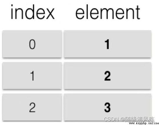
Series: Is a one-dimensional labeled data type object , Can save any data type (int,str,float,python object), Contains data labels , Known as the index
(1) Create... From a list
# 1、 adopt list establish
s1 = pd.Series([1,2,3,4,5])
s1
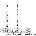
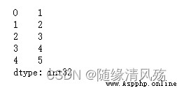
(2) Create... From an array
# 2、 Create... From an array
arr1= np.arange(1,6)
s2 = pd.Series(arr1)
print(s2)
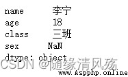
(3) Create... From a dictionary
# 3、 Create... From a dictionary
dict = {
'name':' Lining ','age':18,'class':' Class three '}
s3 = pd.Series(dict,index = ['name','age','class','sex'])
s3
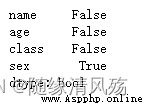
(1) A null value judgment
# isnull and not null Detect missing values
s3.isnull()
(2) get data
How to get data : Indexes , Subscript , Tag name
# 1、 Index get data
print(s3.index)
print(s3.values)
# 2、 Subscript get data
print(s3[1:3])
# 3、 Tag name get data
print(s3['age':'class'])
 The difference between label slice and subscript slice
Label slice : Contains end data
Index slice : Does not contain end data
(3) The correspondence between index and data
The correspondence between the index and the data is not affected by the operation results
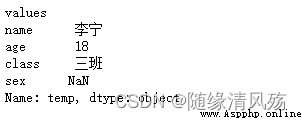
(4)name attribute
s3.name = "temp" # Object name
s3.index.name = 'values' # Object index name
s3
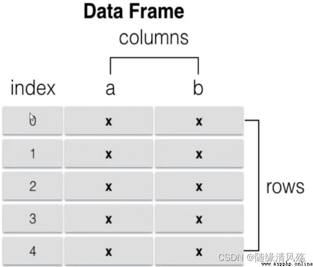
DataFrame It's a Tabular form Data structure of , It has an ordered set of columns , Each column can be a different type of index value ,DataFrame There are both row and column indexes , It can be seen as made up of series A dictionary made up of , Data is stored in a two-dimensional structure
# Array 、 A dictionary constructed of lists or tuples DataFrame
data = {
'a':[1,2,3,4],
'b':(5,6,7,8),
'c':np.arange(9,13)}
frame = pd.DataFrame(data)
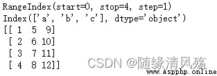
# Related properties
print(frame.index)
print(frame.columns)
print(frame.values)
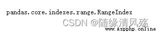
1、Series and DataFrame All the indexes in are index object
2、 The index object cannot be changed , Ensure data security
ps = pd.Series(range(5))
pd = pd.DataFrame(np.arange(9).reshape(3,3),index = ['a','b','c'],columns = ['A','B','C'])
type(ps.index)
 Common index types
:1、Index - Indexes
:2、Inet64index - Integer index
:3、MultiIndex - Hierarchical index
:4、DatetiemIndex - Time stamp index
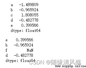
(1) Re index
reindex: Reorder the index , Create a new object that matches the new index
s = pd.Series(np.random.randn(5),index=['a','b','c','d','e'])
print(s)
s.reindex(['e','b','f','d'])
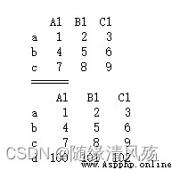
(2) increase
1、 Add data to the original data structure
2、 Add data to the new data structure
s = pd.Series(np.random.randn(5),index=['a','b','c','d','e'])
s['f'] = 100
print(s)
import numpy as np
import pandas as pd
df = pd.DataFrame(np.arange(1,10).reshape(3,3),index=['a','b','c'],columns = ['A1','B1','C1'])
print(df)
print("======")
df['D1'] = np.arange(100,103)
df2 = df
print(df2)
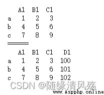
import numpy as np
import pandas as pd
df = pd.DataFrame(np.arange(1,10).reshape(3,3),index=['a','b','c'],columns = ['A1','B1','C1'])
print(df)
print("======")
df.loc['d'] = np.arange(100,103)
df2 = df
print(df2)
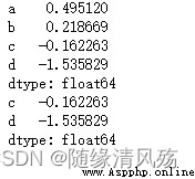
(3) Delete
1、del: Delete , Will change the original structure
2、drop: Delete data on axis , Create new objects
# Delete
ps = pd.Series(np.random.randn(5),index=['a','b','c','d','e'])
del ps['e']
print(ps)
ps2 = ps.drop(['a','b'])
print(ps2)
import numpy as np
import pandas as pd
pd = pd.DataFrame(np.random.randn(9).reshape(3,3),columns=['a','b','c'])
print(pd)
# Delete column
pd1 = pd.drop(['c'],axis=1)
print(pd1)
# Delete row
pd2 = pd.drop(2)
print(pd2)
(4) Change
1、 Modify the column : object . Indexes , object . Column
2、 Modify the line : Tag Index loc
import numpy as np
import pandas as pd
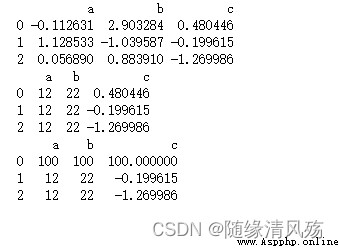
pd = pd.DataFrame(np.random.randn(9).reshape(3,3),columns=['a','b','c'])
print(pd)
# Modify the column
pd['a'] = 12
pd.b = 22
print(pd)
# Modify the line
pd.loc[0] = 100
print(pd)
(5) check
1、 Row index
2、 Slice indices : Position slice , Label slice
3、 Discontinuous index
import numpy as np
import pandas as pd
ps = pd.Series(np.random.randn(5),index=['a','b','c','d','e'])
# Row index
print(ps['a'])
# Location slice index
print(ps[1:3])
# Label slice index , Include termination index
print(ps['a':'c'])
# Discontinuous index
print(ps[['a','c']])
# Boolean index
print(ps[ps>0])
1、loc Tag Index : Index based on tag name pd.loc[2:3,'a']
2、iloc Location index : Index based on index number
3、ix Label and location mixed index : Just know
import numpy as np
import pandas as pd
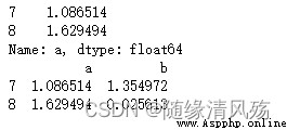
pd = pd.DataFrame(np.random.randn(9).reshape(3,3),index = [7,8,9],columns=['a','b','c'])
# Tag Index - The first parameter indexes the row , The second parameter is the column
print(pd.loc[7:8,'a'])
# Location index - Two parameters , The ranks of
print(pd.iloc[0:2,0:2])

import numpy as np
import pandas as pd
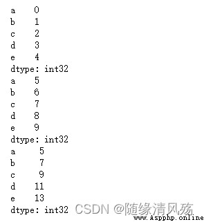
s1 = pd.Series(np.arange(5),index=['a','b','c','d','e'])
s2 = pd.Series(np.arange(5,10),index=['a','b','c','d','e'])
print(s1)
print(s2)
print(s1+s2)
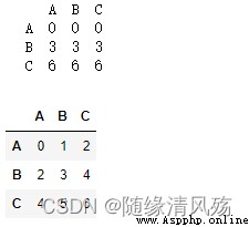
DataFrame and Series Mixed operations :Series The row index of matches DataFrame Column index for broadcast operation ,index Attributes can be computed along columns
import pandas as pd
import numpy as np
df = pd.DataFrame(np.arange(9).reshape(3,3),index = ['A','B','C'],columns=['A','B','C'])
ds = df.iloc[0]
# Row operation , Column broadcast
print(df-ds)
# Column operation , Line broadcast
df.sub(ds,axis = 'index')
Operational rules : Index matching operation
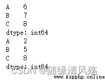
(1)apply function
apply: Apply functions to rows or columns
import pandas as pd
import numpy as np
df = pd.DataFrame(np.arange(9).reshape(3,3),index = ['A','B','C'],columns=['A','B','C'])
f = lambda x:x.max()
# Apply on line , Perform column operations
print(df.apply(f))
# Apply to columns , Perform line operations
print(df.apply(f,axis=1))
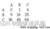
(2)applymap function
applymap: Apply the function to each data
import pandas as pd
import numpy as np
df = pd.DataFrame(np.arange(9).reshape(3,3),index = ['A','B','C'],columns=['A','B','C'])
f = lambda x:x**2
print(df.applymap(f))
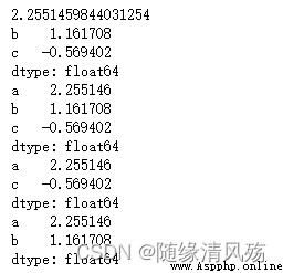
(3) Sort
 Index sort :sort_index(ascending,axis)
Sort by value :sort_values(by,sacending,axis)
import pandas as pd
import numpy as np
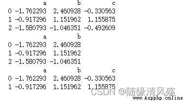
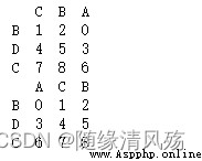
df = pd.DataFrame(np.arange(9).reshape(3,3),index = ['B','D','C'],columns=['A','C','B'])
# Sort by row index
print(df.sort_index(ascending=False,axis=1))
# Sort by column value
print(df.sort_values(by = 'A'))
(4) Unique values and member properties
(5) Handling missing values
import pandas as pd
import numpy as np
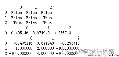
df = pd.DataFrame([np.random.randn(3),[1,2,np.nan],[np.nan,4,np.nan]])
# 1、 Determine if there are missing values
print(df.isnull())
# 2、 Discard missing data , The default discards rows
print(df.dropna())
# 3、 Fill in missing data
print(df.fillna(-100))
Hierarchical index **: In the input index Index when , The input is made up of two subunits list Composed of list, The first one list It's the outer index , the second list It's the inner index .**
effect : Use the hierarchical index with the primary index of different levels , High dimensional arrays can be converted to Series or DataFrame Opposite form
Example
import pandas as pd
import numpy as np
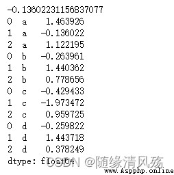
ser_obj = pd.Series(np.random.randn(12),index=[
['a', 'a', 'a', 'b', 'b', 'b', 'c', 'c', 'c', 'd', 'd', 'd'],
[0, 1, 2, 0, 1, 2, 0, 1, 2, 0, 1, 2]
])
# Select a subset
''' Get data from index . Because now there are two layers of indexes , When getting data through the outer index , You can directly use the tag of the outer index to get . When you want to get data through the inner index , stay list Pass in two elements , The former refers to the outer index to be selected , The latter represents the inner index to be selected . '''
print(ser_obj['a',1])
# Exchange inner and outer layers
print(ser_obj.swaplevel())
Statistical calculation : Calculate by column by default
import pandas as pd
import numpy as np
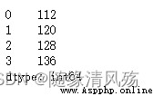
df = pd.DataFrame(np.arange(32).reshape(8,4))
# selection
df.sum()
 The average :np.mean()
The sum of the :np.sum()
Median :np.median()
Maximum :np.max()
minimum value :np.min()
The frequency of ( Count ): np.size()
variance :np.var()
Standard deviation :np.std()
The product of :np.prod()
covariance : np.cov(x, y)
Skewness coefficient (Skewness): skew(x)
Kurtosis coefficient (Kurtosis): kurt(x)
Normality test results : normaltest(np.array(x))
Four percentile :np.quantile(q=[0.25, 0.5, 0.75], interpolation=“linear”)
Four percentile :describe() – Show 25%, 50%, 75% Data on location
correlation matrix (Spearman/ Person/ Kendall) The correlation coefficient : x.corr(method=“person”))
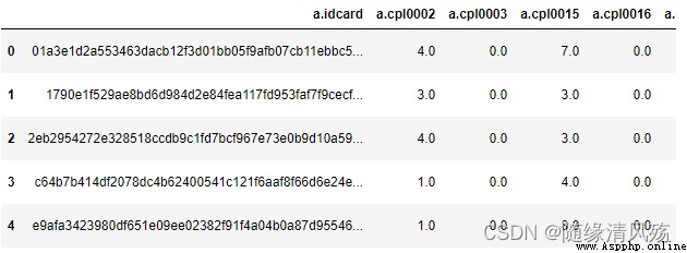
Read csv file read_csv(file_path or buf,usecols,encoding):file_path: File path ,usecols: Specify the column name to read ,encoding: code
Example
data = pd.read_csv('D:/jupyter_notebook/bfms_w2_out.csv',encoding='utf8')
data.head()
pd.merge:(left, right, how='inner',on=None,left\_on=None, right\_on=None \)
left: On the left side of the merger DataFrame
right: When merging, the one on the right DataFrame
how: The way to merge , Default 'inner', 'outer', 'left', 'right'
on: Column names that need to be merged , There must be a list on both sides , And left and right The intersection of column names in is used as the join key
left\_on: left Dataframe Column used as a join key in
right\_on: right Dataframe Column used as a join key in
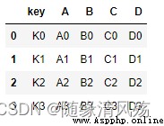
* Internal connection inner: Join the intersection of the keys in both tables
import pandas as pd
import numpy as np
left = pd.DataFrame({
'key': ['K0', 'K1', 'K2', 'K3'],
'A': ['A0', 'A1', 'A2', 'A3'],
'B': ['B0', 'B1', 'B2', 'B3']})
right = pd.DataFrame({
'key': ['K0', 'K1', 'K2', 'K3'],
'C': ['C0', 'C1', 'C2', 'C3'],
'D': ['D0', 'D1', 'D2', 'D3']})
pd.merge(left,right,on='key') # Specify the connection key key
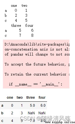
concat: You can specify the axis to merge horizontally or vertically
df1 = pd.DataFrame(np.arange(6).reshape(3,2),index=list('abc'),columns=['one','two'])
df2 = pd.DataFrame(np.arange(4).reshape(2,2)+5,index=list('ac'),columns=['three','four'])
print(df1)
print(df2)
pd.concat([df1,df2],axis='columns') # Appoint axis=1 Connect
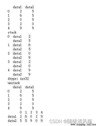
stack:stack The function takes data from ” Table structure “ become ” Curly bracket structure “, Change its row index into column index
unstack:unstack Function to transfer data from ” Curly bracket structure “ become ” Table structure “, That is to change the column index of one layer into a row index .
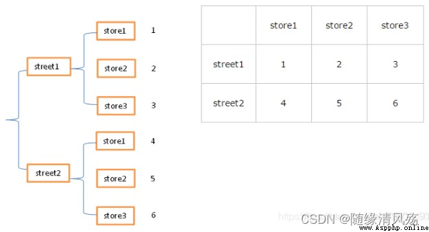
import numpy as np
import pandas as pd
df_obj = pd.DataFrame(np.random.randint(0,10, (5,2)), columns=['data1', 'data2'])
print(df_obj)
print("stack")
stacked = df_obj.stack()
print(stacked)
print("unstack")
# Default operation inner index
print(stacked.unstack())
# adopt level Specifies the level of the operation index
print(stacked.unstack(level=0))