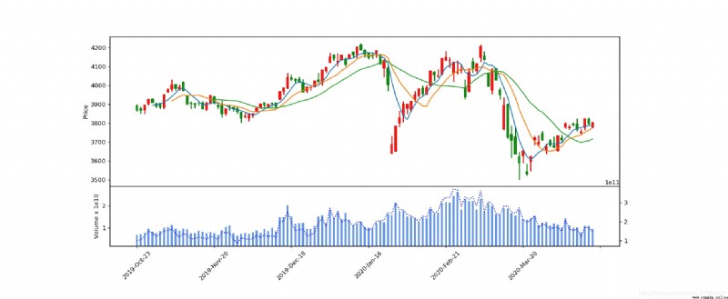
The first three times have been improved and explored step by step , Used on the final system presentation K The line chart must conform to the habits of China's securities trading , Red means up , Green means falling .
In the final system implementation, it is called in the form of function .
Function as follows
#path Is the path of the data ,K Represents the last stored file name
def Drawmpf1(path,k):
# Data processing
df= pd.read_csv(path)
df.columns = ['Date','Open','Close','High', 'Low','Volume',"Money"]
df.head()
df =df.set_index(["Date"])
df.index = pd.DatetimeIndex(df.index)# Multiple indexes can be directly operated
open1=df['Open']
high2=df['High']
low3=df['Low']
close4=df['Close']
volume5=df['Volume']
money6=df['Money']
data=pd.concat([open1,high2,low3,close4,volume5,money6],keys=['Open', 'High','Low' ,'Close','Volume',"Money"],axis=1)
# Image rendering
apds = [mpf.make_addplot((df["Money"][-120:-1]),panel='lower',color='b',linestyle='dotted')]
save = dict(fname=k+".jpg",dpi=120,pad_inches=0)
# Red up , Green down
mc = mpf.make_marketcolors(up='r',down='g',edge='inherit',
wick={
'up':'r','down':'g'},
volume='cornflowerblue',
ohlc='i'
)
s = mpf.make_mpf_style(marketcolors=mc)
mpf.plot(data.iloc[-120:-1],addplot=apds,figscale=1,mav=(5,10,20),volume=True,figratio=(17,7),type='candle', style=s,savefig=save)
#
Call function
1. Call directly
Drawmpf1(path,'SAVE')
The pictures will be stored in the corresponding directory .
2. Cycle call
Process multiple files at once
# Folder Directory
l=["ETF/"]
for i in l:
for k in os.listdir(i):
path=i+k
# Output corresponding path
print(path)
Drawmpf2(path,k)
Use mplfinance draw K End of line diagram , It is really simple and convenient to compare with the previous ones .