Case practice
Problem description one : Count the number of different types of emergencies in these data .
Scheme 1 :set Method
Option two :for Traverse the whole DataFrame
Option three : Add a column , Then the classification Groupby
Time series analysis
( One ) Generate a time range
( Two ) stay DataFrame Use time series in
( 3、 ... and )pandas Resampling
Downsampling ( High frequency data to low frequency data ):
L sampling ( Low frequency data to high frequency data )
( One ) Data initialization operation :
( Two ) According to the statistics 911 Number of calls in different months in the data
( 3、 ... and ) Visual analysis —— drawing
Expand practice ——911 Changes in the number of different types of calls in different months in the data
About PM2.5 Of Demo
Now we have 2015 To 2017 year 25 Ten thousand 911 Emergency call data , Please count out these data Number of different types of emergencies , If we still want to figure out Different types in different months Changes in the number of emergency calls , What should be done ?
Data sources :https://www.kaggle.com/mchirico/montcoalert/data
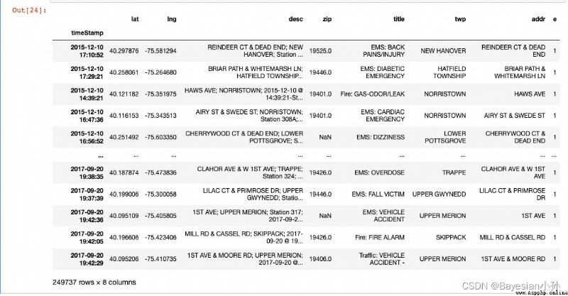
First , Import some basic data analysis packages , Read data information , View the data head and info()
import pandas as pd
import numpy as np
from matplotlib import pyplot as plt
df = pd.read_csv("./911.csv")
print(df.head(3))
print(df.info())
>>> df.head()
lat lng desc \
0 40.297876 -75.581294 REINDEER CT & DEAD END; NEW HANOVER; Station ...
1 40.258061 -75.264680 BRIAR PATH & WHITEMARSH LN; HATFIELD TOWNSHIP...
2 40.121182 -75.351975 HAWS AVE; NORRISTOWN; 2015-12-10 @ 14:39:21-St...
zip title timeStamp twp \
0 19525.0 EMS: BACK PAINS/INJURY 2015-12-10 17:10:52 NEW HANOVER
1 19446.0 EMS: DIABETIC EMERGENCY 2015-12-10 17:29:21 HATFIELD TOWNSHIP
2 19401.0 Fire: GAS-ODOR/LEAK 2015-12-10 14:39:21 NORRISTOWN
addr e
0 REINDEER CT & DEAD END 1
1 BRIAR PATH & WHITEMARSH LN 1
2 HAWS AVE 1
>>> df.info()
<class 'pandas.core.frame.DataFrame'>
RangeIndex: 249737 entries, 0 to 249736
Data columns (total 9 columns):
# Column Non-Null Count Dtype
--- ------ -------------- -----
0 lat 249737 non-null float64
1 lng 249737 non-null float64
2 desc 249737 non-null object
3 zip 219391 non-null float64
4 title 249737 non-null object
5 timeStamp 249737 non-null object
6 twp 249644 non-null object
7 addr 249737 non-null object
8 e 249737 non-null int64
dtypes: float64(3), int64(1), object(5)
memory usage: 17.1+ MBWe need to title Cut the contents inside , Extract [EMS,Fire,Traffic] The content of .
data_1 = df["title"].str.split(":").tolist()
data_1[0:5]
>>>
[['EMS', ' BACK PAINS/INJURY'],
['EMS', ' DIABETIC EMERGENCY'],
['Fire', ' GAS-ODOR/LEAK'],
['EMS', ' CARDIAC EMERGENCY'],
['EMS', ' DIZZINESS']]
Next, I'll extract data_1 in category Information about .
cate_list = list(set(i[0] for i in data_1))
cate_list
>>>
['Fire', 'EMS', 'Traffic']
At this time, we have several ways to According to the statistics Number of different types of emergencies .
zeros_df = pd.DataFrame(np.zeros((df.shape[0],len(cate_list))),columns=cate_list)
for cate in cate_list:
zeros_df[cate][df["title"].str.contains(cate)] = 1
# break
print(zeros_df)
sum_ret = zeros_df.sum(axis=0)
print(sum_ret)
>>>
Fire EMS Traffic
0 0.0 1.0 0.0
1 0.0 1.0 0.0
2 1.0 0.0 0.0
3 0.0 1.0 0.0
4 0.0 1.0 0.0
... ... ... ...
249732 0.0 1.0 0.0
249733 0.0 1.0 0.0
249734 0.0 1.0 0.0
249735 1.0 0.0 0.0
249736 0.0 0.0 1.0
[249737 rows x 3 columns]
Fire 37432.0
EMS 124844.0
Traffic 87465.0
dtype: float6
then sum Just a moment .
zeros_df.sum(axis = 0)
>>>
Fire 37432.0
EMS 124844.0
Traffic 87465.0
dtype: float64Go through all the lists directly , This way is quite slow .
for i in range(df.shape[0]):
zeros_df.loc[i,data_1[i][0]] =1
pass
print(zeros_df)
>>>
Fire EMS Traffic
0 0.0 1.0 0.0
1 0.0 1.0 0.0
2 1.0 0.0 0.0
3 0.0 1.0 0.0
4 0.0 1.0 0.0
... ... ... ...
249732 0.0 1.0 0.0
249733 0.0 1.0 0.0
249734 0.0 1.0 0.0
249735 1.0 0.0 0.0
249736 0.0 0.0 1.0
[249737 rows x 3 columns]
zeros_df.sum(axis = 0)
zeros_df.sum(axis = 0) Add a column , then groupby, Last count Count it .
cate_list = [i[0] for i in data_1]
df["cate"] = pd.DataFrame(np.array(cate_list).reshape((df.shape[0],1)))
print(df.groupby(by="cate").count()["title"])
>>>
cate
EMS 124840
Fire 37432
Traffic 87465
Name: title, dtype: int64
Problem description 2 : Statistics of different months , Changes in different types of emergency calls .
This involves time series analysis .
stay pandas Processing time series in is very simple
pd.date_range(start=None, end=None, periods=None, freq='D')
start and end as well as freq Coordination can produce start and end Range Internal to frequency freq A set of time indexes
start and periods as well as freq Coordination can be generated from start The starting frequency is freq Of periods individual Time index
four parameters: start, end, periods, and freq, exactly three must be specified
Four parameters , You must specify at least three of them .
import pandas as pd
pd.date_range(start="20170909",end = "20180908",freq = "M")
>>>
DatetimeIndex(['2017-09-30', '2017-10-31', '2017-11-30', '2017-12-31',
'2018-01-31', '2018-02-28', '2018-03-31', '2018-04-30',
'2018-05-31', '2018-06-30', '2018-07-31', '2018-08-31'],
dtype='datetime64[ns]', freq='M')
pd.date_range(start="20170909",periods = 5,freq = "D")
>>>
DatetimeIndex(['2017-09-09', '2017-09-10', '2017-09-11', '2017-09-12',
'2017-09-13'],
dtype='datetime64[ns]', freq='D')
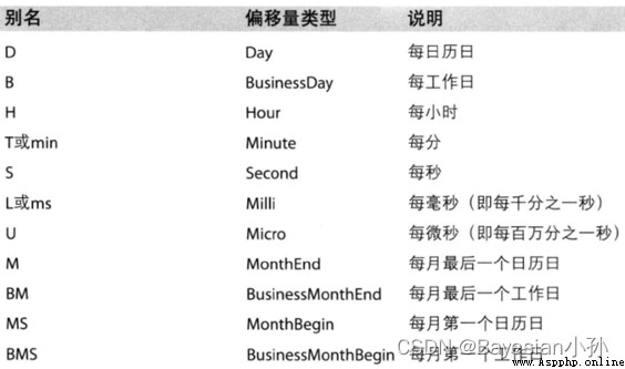
freq: Is the frequency of time .
More abbreviations for frequency
import numpy as np
index=pd.date_range("20170101",periods=10)
df = pd.DataFrame(np.random.rand(10),index=index)
df
>>>
0
2017-01-01 0.090949
2017-01-02 0.996337
2017-01-03 0.737334
2017-01-04 0.405381
2017-01-05 0.743721
2017-01-06 0.681303
2017-01-07 0.606283
2017-01-08 0.917397
2017-01-09 0.167316
2017-01-10 0.155164
Go back to the beginning 911 In the case of data , We can use pandas The method provided converts a time string into a time series
df["timeStamp"] = pd.to_datetime(df["timeStamp"],format="")format In most cases, parameters can be left blank , But for pandas Unformatted time string , We can Use this parameter , For example, include Chinese .
So here comes the question :
Now we need to count the number of times in each month or quarter. What should we do ?
Resampling : It refers to the transformation of time series from One frequency is converted to another frequency Processing process , Convert high frequency data into low frequency data Downsampling , Low frequency is converted to high frequency L sampling .pandas Provides a resample To help us achieve frequency conversion
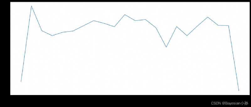
1. According to the statistics 911 Changes in the number of calls in different months in the data .
2. According to the statistics 911 Changes in the number of different types of calls in different months in the data .
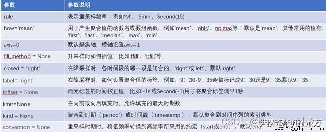
pandas.DataFrame.resample
pandas.DataFrame.resample() This function is mainly used for The time series Do frequency conversion , The function prototype is as follows :
DataFrame.resample(rule, how=None, axis=0, fill_method=None, closed=None, label=None, convention='start', kind=None, loffset=None, limit=None, base=0, on=None, level=None)
import pandas as pd
import numpy as np
index=pd.date_range('20190115','20190125',freq='D')
data1=pd.Series(np.arange(len(index)),index=index)
data1
>>>
2019-01-15 0
2019-01-16 1
2019-01-17 2
2019-01-18 3
2019-01-19 4
2019-01-20 5
2019-01-21 6
2019-01-22 7
2019-01-23 8
2019-01-24 9
2019-01-25 10
Freq: D, dtype: int64
data1.resample(rule='3D').sum() >>> 2019-01-15 3 2019-01-18 12 2019-01-21 21 2019-01-24 19 Freq: 3D, dtype: int64 data1.resample(rule='3D').mean() >>> 2019-01-15 1.0 2019-01-18 4.0 2019-01-21 7.0 2019-01-24 9.5 Freq: 3D, dtype: float64
label This parameter controls the value of the aggregate tag after grouping . stay label by right Under the circumstances , Take the value on the right side of the sub box as the new label .
The process of downsampling is demonstrated above , Let's demonstrate the process of liter sampling , According to the definition of liter sampling , We just need to resample Function to change the frequency , However, unlike downsampling, the number of new frequencies after upsampling is null , So resample Also provided 3 There are three ways to fill , Let's use code to demonstrate :
The three filling methods are :
ffill( Take the previous value )
bfill( Take the following value )
interpolate( Linear value )
data1.resample(rule='12H').asfreq()
>>>
2019-01-15 00:00:00 0.0
2019-01-15 12:00:00 NaN
2019-01-16 00:00:00 1.0
2019-01-16 12:00:00 NaN
2019-01-17 00:00:00 2.0
2019-01-17 12:00:00 NaN
2019-01-18 00:00:00 3.0
2019-01-18 12:00:00 NaN
2019-01-19 00:00:00 4.0
2019-01-19 12:00:00 NaN
2019-01-20 00:00:00 5.0
2019-01-20 12:00:00 NaN
2019-01-21 00:00:00 6.0
2019-01-21 12:00:00 NaN
2019-01-22 00:00:00 7.0
2019-01-22 12:00:00 NaN
2019-01-23 00:00:00 8.0
2019-01-23 12:00:00 NaN
2019-01-24 00:00:00 9.0
2019-01-24 12:00:00 NaN
2019-01-25 00:00:00 10.0
Freq: 12H, dtype: float64
The original daily data is upsampled to 6 Hour hour , Many null values will be generated , For this null value resample Provides 3 Ways of planting , Respectively ffill( Take the previous value )、bfill( Take the following value )、interpolate( Linear value ), Here we test separately , as follows :
(1) stay ffill When no parameters are passed in , be-all NAN Be filled with , Here we can enter the number , So as to specify the number of null values to be filled .
data1.resample(rule='12H').ffill()
# Forward filling , take NAN Fill in the previous values
2019-01-15 00:00:00 0
2019-01-15 12:00:00 0
2019-01-16 00:00:00 1
2019-01-16 12:00:00 1
2019-01-17 00:00:00 2
2019-01-17 12:00:00 2
2019-01-18 00:00:00 3
2019-01-18 12:00:00 3
2019-01-19 00:00:00 4
2019-01-19 12:00:00 4
2019-01-20 00:00:00 5
2019-01-20 12:00:00 5
2019-01-21 00:00:00 6
2019-01-21 12:00:00 6
2019-01-22 00:00:00 7
2019-01-22 12:00:00 7
2019-01-23 00:00:00 8
2019-01-23 12:00:00 8
2019-01-24 00:00:00 9
2019-01-24 12:00:00 9
2019-01-25 00:00:00 10
Freq: 12H, dtype: int64
data1.resample(rule='12H').ffill(2)
>>>
2019-01-15 00:00:00 0
2019-01-15 12:00:00 1
2019-01-16 00:00:00 1
2019-01-16 12:00:00 2
2019-01-17 00:00:00 2
2019-01-17 12:00:00 3
2019-01-18 00:00:00 3
2019-01-18 12:00:00 4
2019-01-19 00:00:00 4
2019-01-19 12:00:00 5
2019-01-20 00:00:00 5
2019-01-20 12:00:00 6
2019-01-21 00:00:00 6
2019-01-21 12:00:00 7
2019-01-22 00:00:00 7
2019-01-22 12:00:00 8
2019-01-23 00:00:00 8
2019-01-23 12:00:00 9
2019-01-24 00:00:00 9
2019-01-24 12:00:00 10
2019-01-25 00:00:00 10
Freq: 12H, dtype: int64
data1.resample(rule='12H').bfill()
>>>
2019-01-15 00:00:00 0
2019-01-15 12:00:00 1
2019-01-16 00:00:00 1
2019-01-16 12:00:00 2
2019-01-17 00:00:00 2
2019-01-17 12:00:00 3
2019-01-18 00:00:00 3
2019-01-18 12:00:00 4
2019-01-19 00:00:00 4
2019-01-19 12:00:00 5
2019-01-20 00:00:00 5
2019-01-20 12:00:00 6
2019-01-21 00:00:00 6
2019-01-21 12:00:00 7
2019-01-22 00:00:00 7
2019-01-22 12:00:00 8
2019-01-23 00:00:00 8
2019-01-23 12:00:00 9
2019-01-24 00:00:00 9
2019-01-24 12:00:00 10
2019-01-25 00:00:00 10
Freq: 12H, dtype: int64
data1.resample(rule='12H').interpolate()
# Linear filling
>>>
2019-01-15 00:00:00 0.0
2019-01-15 12:00:00 0.5
2019-01-16 00:00:00 1.0
2019-01-16 12:00:00 1.5
2019-01-17 00:00:00 2.0
2019-01-17 12:00:00 2.5
2019-01-18 00:00:00 3.0
2019-01-18 12:00:00 3.5
2019-01-19 00:00:00 4.0
2019-01-19 12:00:00 4.5
2019-01-20 00:00:00 5.0
2019-01-20 12:00:00 5.5
2019-01-21 00:00:00 6.0
2019-01-21 12:00:00 6.5
2019-01-22 00:00:00 7.0
2019-01-22 12:00:00 7.5
2019-01-23 00:00:00 8.0
2019-01-23 12:00:00 8.5
2019-01-24 00:00:00 9.0
2019-01-24 12:00:00 9.5
2019-01-25 00:00:00 10.0
Freq: 12H, dtype: float64
Set the index of the original data to the time index value , Do the following .
import pandas as pd
import numpy as np
from matplotlib import pyplot as plt
df = pd.read_csv("./911.csv")
df["timeStamp"] = pd.to_datetime(df["timeStamp"])
df.set_index("timeStamp",inplace=True)
df
>>>
count_by_month = df.resample("M").count()["title"]
print(count_by_month)
>>>
timeStamp
2015-12-31 7916
2016-01-31 13096
2016-02-29 11396
2016-03-31 11059
2016-04-30 11287
2016-05-31 11374
2016-06-30 11732
2016-07-31 12088
2016-08-31 11904
2016-09-30 11669
2016-10-31 12502
2016-11-30 12091
2016-12-31 12162
2017-01-31 11605
2017-02-28 10267
2017-03-31 11684
2017-04-30 11056
2017-05-31 11719
2017-06-30 12333
2017-07-31 11768
2017-08-31 11753
2017-09-30 7276
Freq: M, Name: title, dtype: int64
# drawing
_x = count_by_month.index
_y = count_by_month.values
_x = [i.strftime("%Y%m%d") for i in _x]
plt.figure(figsize=(20,8),dpi=80)
plt.plot(range(len(_x)),_y)
plt.xticks(range(len(_x)),_x,rotation=45)
plt.show()
import pandas as pd
import numpy as np
from matplotlib import pyplot as plt
# Convert the time string to time type and set it as index
df = pd.read_csv("./911.csv")
df["timeStamp"] = pd.to_datetime(df["timeStamp"])
# Add columns , Indicates classification
temp_list = df["title"].str.split(": ").tolist()
cate_list = [i[0] for i in temp_list]
# print(np.array(cate_list).reshape((df.shape[0],1)))
df["cate"] = pd.DataFrame(np.array(cate_list).reshape((df.shape[0],1)))
df.set_index("timeStamp",inplace=True)
print(df.head(1))
plt.figure(figsize=(20, 8), dpi=80)
# grouping
for group_name,group_data in df.groupby(by="cate"):
# Draw different categories
count_by_month = group_data.resample("M").count()["title"]
# drawing
_x = count_by_month.index
print(_x)
_y = count_by_month.values
_x = [i.strftime("%Y%m%d") for i in _x]
plt.plot(range(len(_x)), _y, label=group_name)
plt.xticks(range(len(_x)), _x, rotation=45)
plt.legend(loc="best")
plt.show()
>>>
lat lng \
timeStamp
2015-12-10 17:10:52 40.297876 -75.581294
desc \
timeStamp
2015-12-10 17:10:52 REINDEER CT & DEAD END; NEW HANOVER; Station ...
zip title twp \
timeStamp
2015-12-10 17:10:52 19525.0 EMS: BACK PAINS/INJURY NEW HANOVER
addr e cate
timeStamp
2015-12-10 17:10:52 REINDEER CT & DEAD END 1 EMS
DatetimeIndex(['2015-12-31', '2016-01-31', '2016-02-29', '2016-03-31',
'2016-04-30', '2016-05-31', '2016-06-30', '2016-07-31',
'2016-08-31', '2016-09-30', '2016-10-31', '2016-11-30',
'2016-12-31', '2017-01-31', '2017-02-28', '2017-03-31',
'2017-04-30', '2017-05-31', '2017-06-30', '2017-07-31',
'2017-08-31', '2017-09-30'],
dtype='datetime64[ns]', name='timeStamp', freq='M')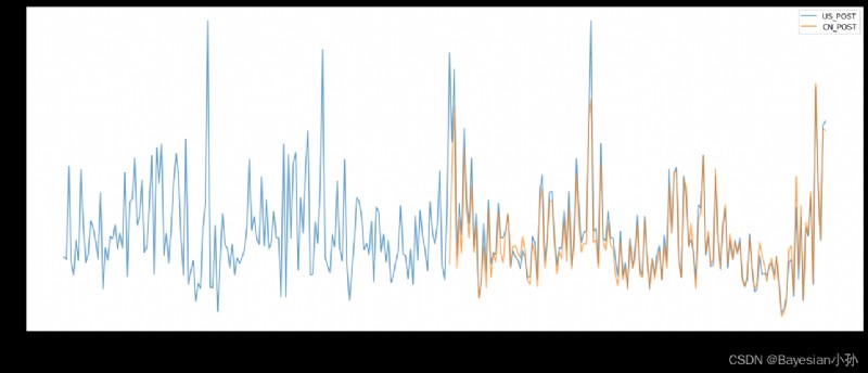
# coding=utf-8
import pandas as pd
from matplotlib import pyplot as plt
file_path = "./PM2.5/BeijingPM20100101_20151231.csv"
df = pd.read_csv(file_path)
# Pass the separated time string through periodIndex The method is transformed into pandas The type of time
period = pd.PeriodIndex(year=df["year"],month=df["month"],day=df["day"],hour=df["hour"],freq="H")
df["datetime"] = period
# print(df.head(10))
# hold datetime Set as index
df.set_index("datetime",inplace=True)
# Down sampling
df = df.resample("7D").mean()
print(df.head())
# Processing missing data , Delete missing data
# print(df["PM_US Post"])
data =df["PM_US Post"]
data_china = df["PM_Nongzhanguan"]
print(data_china.head(100))
# drawing
_x = data.index
_x = [i.strftime("%Y%m%d") for i in _x]
_x_china = [i.strftime("%Y%m%d") for i in data_china.index]
print(len(_x_china),len(_x_china))
_y = data.values
_y_china = data_china.values
plt.figure(figsize=(20,8),dpi=80)
plt.plot(range(len(_x)),_y,label="US_POST",alpha=0.7)
plt.plot(range(len(_x_china)),_y_china,label="CN_POST",alpha=0.7)
plt.xticks(range(0,len(_x_china),10),list(_x_china)[::10],rotation=45)
plt.legend(loc="best")
plt.show()
Be careful :
Separate time strings are passed through periodIndex The method is transformed into pandas The type of time
period=pd.PeriodIndex(year=df["year"],month=df["month"],day=df["day"],hour=df["hour"],freq="H")
df["datetime"] = period
About Resampling For some of the contents of :
http://t.csdn.cn/ViZmt