Preface
Complete code
Low pass filtering
High pass filtering
Result display
Low pass filtering
High pass filtering
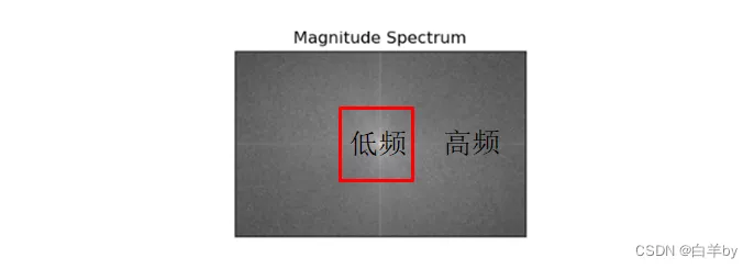
PrefaceIn the last chapter, we explained how to transform the image machine into Fourier transform , Transform the image from time domain to frequency domain , And move the low frequency to the center of the image . Then move the low frequency to the center , The low frequency and high frequency of the image can be separated , Thus, low-pass filtering and high pass filtering are processed .

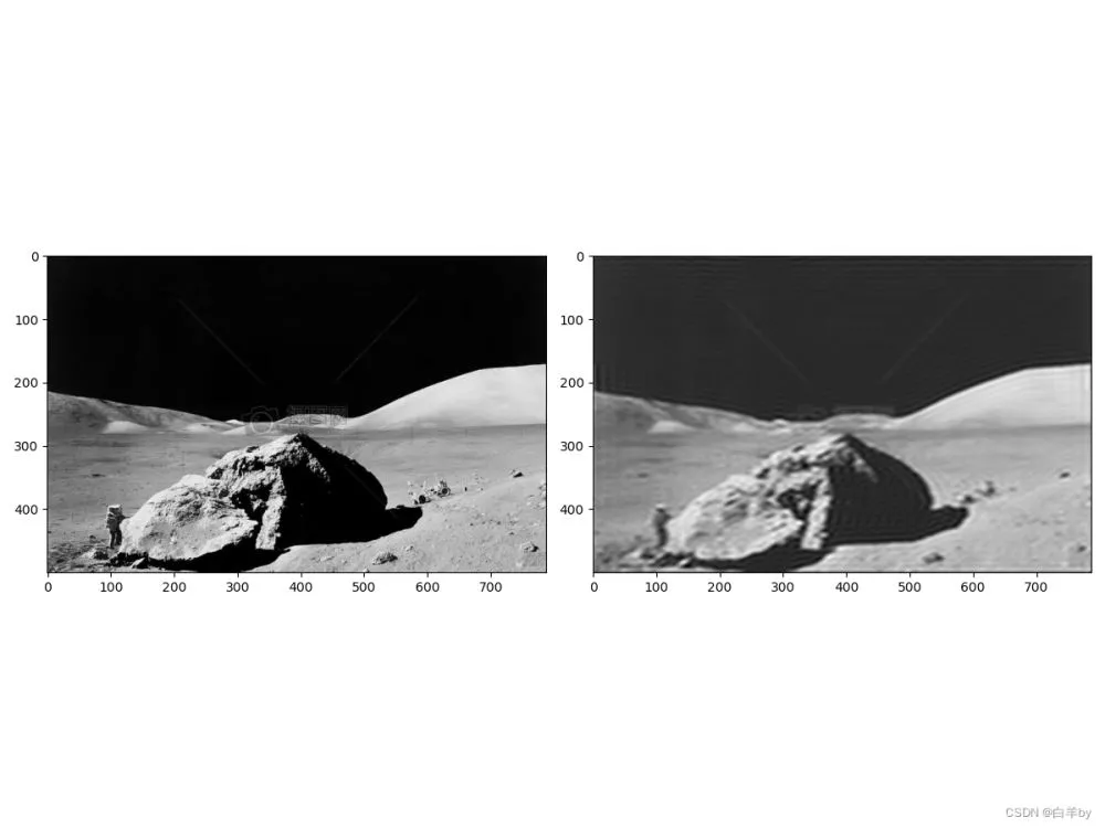
import cv2import numpy as npimport matplotlib.pyplot as plt# cv2.imread() When reading an image , The default is read as RGB Images ,cv2.IMREAD_GRAYSCALE Will be read in the form of a grayscale image img = cv2.imread('./moon.jpg', flags = cv2.IMREAD_GRAYSCALE) # Divide the image by 255 It is to change the image to digital standard fioat32 data img1 = img/255 # Fourier transform , Time domain ——> frequency domain dtf = cv2.dft(img1, flags = cv2.DFT_COMPLEX_OUTPUT) # Move the low frequency wave to the center dft_shift = np.fft.fftshift(dtf) # Low pass filtering h,w = img.shape# The center point of the image is the location of the low-frequency wave h2, w2 = h//2, w//2 mask = np.zeros((h,w,2), dtype=np.uint8)# Select length and width as 100 The low frequency part of the region is 1, The rest is 0mask[h2-50:h2+50,w2-50:w2+50] = 1 # The low frequency part is reserved , The rest of the *0 Filtered out dft_shift*=mask # Inverse Fourier transform , frequency domain ——> Time domain ifft_shift2 = np.fft.ifftshift(dft_shift) result = cv2.idft(ifft_shift2)# Create a display window , Show the original plt.figure(figsize=(12,9))plt.subplot(121)plt.imshow(img, cmap = 'gray')# Create a display window , Display the image after low-pass filtering plt.subplot(122)plt.imshow(result[:,:,0], cmap='gray')plt.show() High pass filtering The main difference between high pass filtering and low-pass filtering is , Low pass filtering is to retain the center of the low-frequency wave and remove the high-frequency wave , High pass filtering is to remove the low-frequency wave in the center and retain the high-frequency wave .
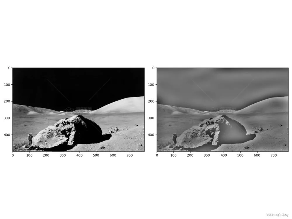
import cv2import numpy as npimport matplotlib.pyplot as plt# cv2.imread() When reading an image , The default is read as RGB Images ,cv2.IMREAD_GRAYSCALE Will be read in the form of a grayscale image img = cv2.imread('./moon.jpg', flags = cv2.IMREAD_GRAYSCALE) # Divide the image by 255 It is to change the image to digital standard fioat32 data img1 = img/255 # Fourier transform , Time domain ——> frequency domain dtf = cv2.dft(img1, flags = cv2.DFT_COMPLEX_OUTPUT) # Move the low frequency wave to the center dft_shift = np.fft.fftshift(dtf)# High pass filtering h,w = img.shape# The center point of the image is the location of the low-frequency wave h2, w2 = h//2, w//2 # Center point # Select length and width as 100 The low frequency part of the region is 0, The other high-frequency parts are 1dft_shift[h2-5:h2+5,w2-5:w2+5] = 0# Inverse Fourier transform , frequency domain ——> Time domain ifft_shift2 = np.fft.ifftshift(dft_shift) result = cv2.idft(ifft_shift2)# Create a display window , Show the original plt.figure(figsize=(12,9))plt.subplot(121)plt.imshow(img, cmap = 'gray')# Create a display window , Display the image after low-pass filtering plt.subplot(122)plt.imshow(result[:,:,0], cmap='gray')plt.show() Result display Changing the size of the filtering area can change the filtering degree , You can modify the relevant parts of the code shown in the figure :


This is about python opencv This is the end of the article on image high pass filtering and low pass filtering , More about python opencv Please search the previous articles of SDN or continue to browse the related articles below. I hope you will support SDN more in the future !