python opencv How to realize high pass filtering and low pass filtering of images

This article mainly introduces “python opencv How to realize high pass filtering and low pass filtering of images ” Knowledge about , Xiaobian shows you the operation process through practical cases , The operation method is simple and fast , Practical , Hope this article “python opencv How to realize high pass filtering and low pass filtering of images ” The article can help you solve problems .

Complete code

Low pass filtering

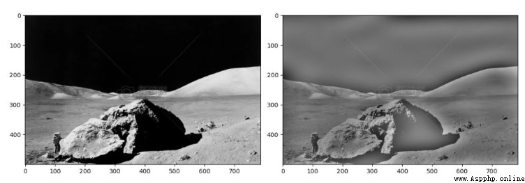
import cv2import numpy as npimport matplotlib.pyplot as plt# cv2.imread() When reading an image , The default is read as RGB Images ,cv2.IMREAD_GRAYSCALE Will be read in the form of a grayscale image img = cv2.imread('./moon.jpg', flags = cv2.IMREAD_GRAYSCALE)  #  Divide the image by 255 It is to change the image to digital standard fioat32 data img1 = img/255 #  Fourier transform , Time domain ——> frequency domain dtf = cv2.dft(img1, flags = cv2.DFT_COMPLEX_OUTPUT)  #  Move the low frequency wave to the center dft_shift = np.fft.fftshift(dtf)  #  Low pass filtering h,w = img.shape#  The center point of the image is the location of the low-frequency wave h3, w2 = h//2, w//2  mask = np.zeros((h,w,2), dtype=np.uint8)#  Select length and width as 100 The low frequency part of the region is 1, The rest is 0mask[h3-50:h3+50,w2-50:w2+50] = 1  #  The low frequency part is reserved , The rest of the *0 Filtered out dft_shift*=mask  #  Inverse Fourier transform , frequency domain ——> Time domain ifft_shift2 = np.fft.ifftshift(dft_shift)  result = cv2.idft(ifft_shift2)#  Create a display window , Show the original plt.figure(figsize=(12,9))plt.subplot(121)plt.imshow(img, cmap = 'gray')#  Create a display window , Display the image after low-pass filtering plt.subplot(122)plt.imshow(result[:,:,0], cmap='gray')plt.show()

High pass filtering

The main difference between high pass filtering and low-pass filtering is , Low pass filtering is to retain the center of the low-frequency wave and remove the high-frequency wave , High pass filtering is to remove the low-frequency wave in the center and retain the high-frequency wave .

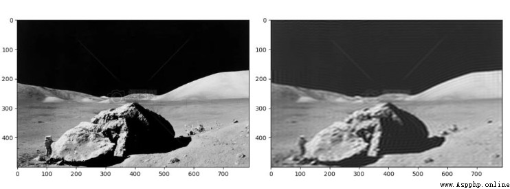
import cv2import numpy as npimport matplotlib.pyplot as plt# cv2.imread() When reading an image , The default is read as RGB Images ,cv2.IMREAD_GRAYSCALE Will be read in the form of a grayscale image img = cv2.imread('./moon.jpg', flags = cv2.IMREAD_GRAYSCALE)  #  Divide the image by 255 It is to change the image to digital standard fioat32 data img1 = img/255 #  Fourier transform , Time domain ——> frequency domain dtf = cv2.dft(img1, flags = cv2.DFT_COMPLEX_OUTPUT)  #  Move the low frequency wave to the center dft_shift = np.fft.fftshift(dtf)#  High pass filtering h,w = img.shape#  The center point of the image is the location of the low-frequency wave h3, w2 = h//2, w//2  #  Center point #  Select length and width as 100 The low frequency part of the region is 0, The other high-frequency parts are 1dft_shift[h3-5:h3+5,w2-5:w2+5] = 0#  Inverse Fourier transform , frequency domain ——> Time domain ifft_shift2 = np.fft.ifftshift(dft_shift)  result = cv2.idft(ifft_shift2)#  Create a display window , Show the original plt.figure(figsize=(12,9))plt.subplot(121)plt.imshow(img, cmap = 'gray')#  Create a display window , Display the image after low-pass filtering plt.subplot(122)plt.imshow(result[:,:,0], cmap='gray')plt.show()

Result display

Changing the size of the filtering area can change the filtering degree , You can modify the relevant parts of the code shown in the figure ：

Low pass filtering

High pass filtering

About “python opencv How to realize high pass filtering and low pass filtering of images ” That's all for , Thanks for reading . If you want to know more about the industry , You can pay attention to the Yisu cloud industry information channel , Xiaobian will update different knowledge points for you every day .