Before that, I introduced the basic content of computer vision , This article formally introduces a widely used content of computer vision , Image retrieval and recognition , The method we use here is from the field of naturallanguageprocessing Bag-of-words Improved from the model Bag of features.
Introducing Bag of features Before the model , Let's first introduce its prototype Bag-of-words Model .
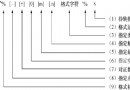
Bagofwords Model , It's also called “ The word bag ”, In Information Retrieval ,Bag of words model Suppose for a text , Ignore its word order and grammar 、 syntax , Think of it as just a collection of words , Or a combination of words , Each word in the text appears independently , It doesn't depend on whether other words appear , In other words, when the author of this article chooses a word at any position, he will not be affected by the previous sentence and choose it independently .
Research shows that , The order of Chinese characters is not definite, which affects reading and reading . For example, after you read this sentence , It's just that the words in the present are all in disorder .
The specific principle can refer to the word bag model in the naive Bayesian algorithm I wrote before : machine learning _5: Naive bayes algorithm
Simply speaking , The word bag model discards the connection between words , Compare each word individually , For example, if two documents have similar content , So they are similar , The most typical example is palindrome , For example, being truthful and not beautiful , Kind words do not believe , It has a different meaning , But if it is word bag detection, it will think that these two sentences are the same sentence .
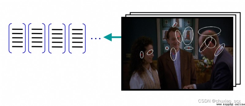
Same as previous feature extraction , We use SIFT The algorithm extracts feature points , Suppose that the number of feature points extracted from each image is fixed 100 individual ( In fact, the number of feature points that can be extracted from each image is different and far greater than 100 individual ), Suppose there is 100 A picture ( The actual number of pictures is far more than this ), So we can collect 1 Ten thousand characteristic points . If we just use this 1 Million feature points as a visual dictionary , For the input feature set , Quantification according to visual dictionary , Convert the input image into visual words (visual words) Frequency histogram .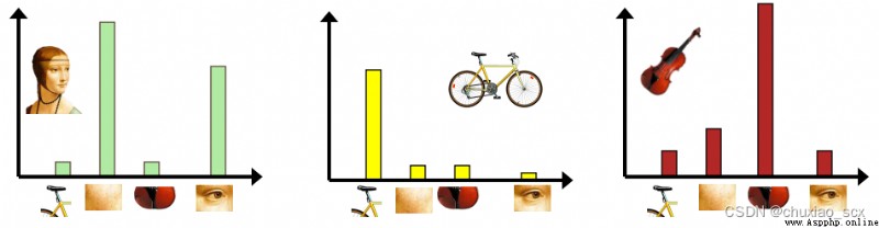
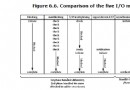
As shown in the figure , Similar to the example in the image , But if we here 1 If ten thousand feature points are used as feature vectors , The frequency histogram of each image becomes very wide , The usage rate is just 1/100. So we use other methods to reduce the number of eigenvectors .
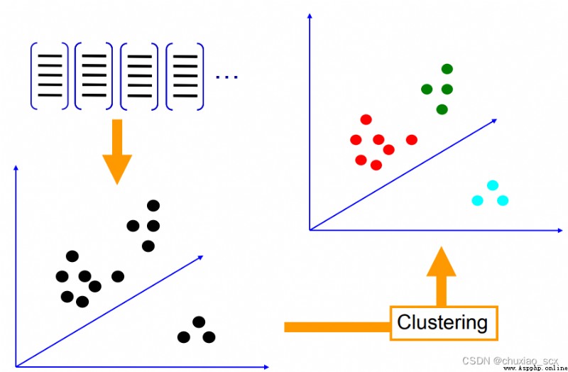
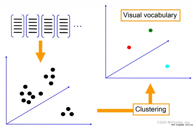
As shown in the figure , Each feature point has RGB Three pixel channels , We convert these feature points into RGB Solid points in color space , Then set it randomly k Cluster centers , Minimize each feature xi The corresponding cluster center mk European distance between , Finally, all the feature points are aggregated k A feature Center , In this way, we can greatly reduce the number of features in the visual dictionary .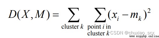
Algorithm flow :
1. Random initialization K In cluster
2. Repeat the following steps until the algorithm converges :
Corresponding to each feature , Assign a value to a center according to the distance relationship / Category
For each category , Recalculate the cluster center according to its corresponding feature set
The problem is obvious ,k It is difficult to determine the value of ,k Too few values , Visual words cannot cover all possible situations ,k Overvalued , Large amount of computation , Easy to overfit
So, with the given image bag-of-features Histogram features , How to realize image classification / Retrieval ?
The of a given input image BOW Histogram , Look up... In the database k The nearest neighbor image , For image classification , According to this k Classification labels of nearest neighbor images , Vote for classification results , When the training data is enough to represent all images , retrieval / The classification effect is good
import pickle
from PCV.imagesearch import vocabulary
from PCV.tools.imtools import get_imlist
from PCV.localdescriptors import sift
# Get image list
imlist = get_imlist("D:\\vscode\\python\\input\\image")
nbr_images = len(imlist)
print('nbr_images:',nbr_images)
# Get feature list
featlist = [imlist[i][:-3]+'sift' for i in range(nbr_images)]
# Extract the image under the folder sift features
for i in range(nbr_images):
sift.process_image(imlist[i], featlist[i])
# Generating words
voc = vocabulary.Vocabulary('Image')
voc.train(featlist, 200, 10)# Called PCV Of vocabulary.py Medium train function
# Save vocabulary
with open('D:\\vscode\\python\\input\\image\\vocabulary.pkl', 'wb') as f:
pickle.dump(voc, f)# Save the generated vocabulary to vocabulary.pkl(f) in
print ('vocabulary is:', voc.name, voc.nbr_words)
import pickle
from PCV.imagesearch import imagesearch
from PCV.localdescriptors import sift
from sqlite3 import dbapi2 as sqlite
from PCV.tools.imtools import get_imlist
# Get image list
imlist = get_imlist("D:\\vscode\\python\\input\\image")
nbr_images = len(imlist)
# Get feature list
featlist = [imlist[i][:-3]+'sift' for i in range(nbr_images)]
# Load vocabulary
with open('D:\\vscode\\python\\input\\image\\vocabulary.pkl', 'rb') as f:
voc = pickle.load(f)
# Create index
indx = imagesearch.Indexer('testImaAdd.db',voc)
indx.create_tables()
# Traverse all images , And project their features onto words
for i in range(nbr_images)[:110]:
locs,descr = sift.read_features_from_file(featlist[i])
indx.add_to_index(imlist[i],descr)
# Commit to database
indx.db_commit()
con = sqlite.connect('testImaAdd.db')
print (con.execute('select count (filename) from imlist').fetchone())
print (con.execute('select * from imlist').fetchone())
import pickle
from PCV.localdescriptors import sift
from PCV.imagesearch import imagesearch
from PCV.geometry import homography
from PCV.tools.imtools import get_imlist
# Load image list
imlist = get_imlist('D:\\vscode\\python\\input\\image')
nbr_images = len(imlist)
# Load feature list
featlist = [imlist[i][:-3]+'sift' for i in range(nbr_images)]
# Load vocabulary
with open('D:\\vscode\\python\\input\\image\\vocabulary.pkl', 'rb') as f:
voc = pickle.load(f)
src = imagesearch.Searcher('testImaAdd.db',voc)
# Query the image index and the number of images returned by the query
q_ind = 1
nbr_results = 5
# Regular query ( Sort the results by Euclidean distance )
res_reg = [w[1] for w in src.query(imlist[q_ind])[:nbr_results]]
print ('top matches (regular):', res_reg)
# load image features for query image
# Load query image features
q_locs,q_descr = sift.read_features_from_file(featlist[q_ind])
fp = homography.make_homog(q_locs[:,:2].T)
# RANSAC model for homography fitting
# Fitting with homography to establish RANSAC Model
model = homography.RansacModel()
rank = {
}
# load image features for result
# Load features of candidate images
for ndx in res_reg[1:]:
locs,descr = sift.read_features_from_file(featlist[ndx]) # because 'ndx' is a rowid of the DB that starts at 1
# get matches
matches = sift.match(q_descr,descr)
ind = matches.nonzero()[0]
ind2 = matches[ind]
tp = homography.make_homog(locs[:,:2].T)
# compute homography, count inliers. if not enough matches return empty list
try:
H,inliers = homography.H_from_ransac(fp[:,ind],tp[:,ind2],model,match_theshold=4)
except:
inliers = []
# store inlier count
rank[ndx] = len(inliers)
# sort dictionary to get the most inliers first
sorted_rank = sorted(rank.items(), key=lambda t: t[1], reverse=True)
res_geom = [res_reg[0]]+[s[0] for s in sorted_rank]
print ('top matches (homography):', res_geom)
# Show query results
imagesearch.plot_results(src,res_reg[:5]) # Regular query
imagesearch.plot_results(src,res_geom[:5]) # The result of the rearrangement
1. Use k-means clustering , In addition to its K And the selection of initial clustering centers , For massive data , The huge input matrix will cause memory overflow and inefficiency .
2. The choice of dictionary size is also a problem , The dictionary is too large , Words lack generality , Sensitive to noise , Large amount of computation , The key is the high dimension of the projected image ; The dictionary is too small , Poor word discrimination , Similar target features cannot be represented .
3. The similarity measure function is used to classify the image features into the corresponding words in the word book , It involves a linear kernel , Collapse distance measure kernel , Selection of histogram cross kernel, etc .