Catalog
Preface
One 、 The basic principle
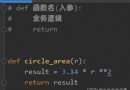
1.1 Introduction to image classification
1.2 Bag-of-words Model
1.3 Bag-of-features Model
1.4 Bag-of-features Algorithm
1.5 Bag-of-features The process
1.6 TF-IDF
Two 、 Code implementation
2.1 Data sets
2.2 Create vocabulary
2.3 Building a database
2.4 Search the database for prime images
2.5 Problems encountered
Reference article
This experiment will refer to Bag-of-words The model implements simple image retrieval operations .
Environmental Science :Pycharm,python3.8.5
Image classification , That is, images are divided into different categories through different image contents , The content-based image classification technology does not need to label the semantic information of the image manually , Instead, the features contained in the image are extracted by computer , And process and analyze the characteristics , Get the classification results .
Common image features are color 、 texture 、 Grayscale Etc . In the process of image classification , The extracted features are not easy to be disturbed by random factors , Effective feature extraction can improve the accuracy of image classification . After feature extraction , Select an appropriate algorithm to create the correlation between image types and visual features , Classify the images .
In the field of image classification , According to the image classification requirements , In general, it can be divided into Scene classification and Target classification There are two kinds of problems .
Scene classification refers to distinguishing images with similar scene features from multiple images .
Object classification refers to the classification of objects in an image The target that appears ( object ) To identify or classify .
Bow The beginning can be understood as a kind of Histogram statistics , It started as a simple document representation method for naturallanguageprocessing and information retrieval .BoW It's just the frequency information , No sequence information .Bow It's choice words Dictionaries , Then count the number of occurrences of each word in the dictionary .
BoW(Bag of Words) Word bag model was originally used in text classification , Representing a document as a feature vector . Its basic idea is to assume that for a text , Ignore its word order and grammar 、 syntax , Just think of it as a collection of words , Each word in the text is independent . Simply put, treat each document as a bag ( Because it's full of words , So it's called word bag ,Bag of words That is why ), Look at the words in the bag , Classify them . If there is a pig in a document 、 Horse 、 cattle 、 sheep 、 The valley 、 land 、 There are more words like tractor , And the bank 、 building 、 automobile 、 There are fewer words like Park , We tend to judge it as a document depicting the countryside , Instead of describing the town .
Bag of Feature It also draws on this idea , Just in the image , What we draw out is no longer one by one word, It is the key feature of the image Feature, So the researchers renamed it Bag of Feature.
Bag of Feature The algorithm flow and classification in retrieval are almost the same , The only difference is , For the original BOF features , Histogram vector , We introduce TF-IDF A weight .
Bag of Feature The essence of is to propose a feature representation method of image
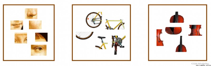
according to Bag of Feature The idea of algorithm , First, we need to find the key features in the image , And these Key features must have a high degree of differentiation . In the actual process , Usually SIFT features .
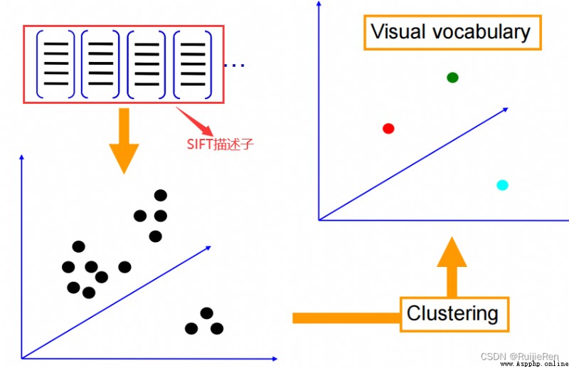
With the characteristics , We will pass these characteristics through clustering algorithm Get a lot of cluster centers . These clustering centers are usually highly representative , such as , For the face , Although different people's eyes 、 The nose and other features are different , But they often have something in common , These clustering centers represent this kind of commonness . We put these clustering centers together , Form a part Visual dictionary (visual vocabulary).
For each in the image SIFT features , We can find the most similar cluster centers in the dictionary , Count the number of occurrences of these cluster centers , You can get a vector representation ( Some articles call it histogram ) These vectors are called Bag. such , For different categories of pictures , This vector should have a large discrimination , Based on this , We can train some classification models (SVM etc. ), And use it to classify the pictures .
Algorithm flow :
(1) Extraction of image features
Feature extraction and description are mainly about Representative And Strong discrimination Of Global or local features Extract from the image , And describe these characteristics .
These characteristics are generally the characteristics with obvious gap between categories , It can be distinguished from other categories , secondly , These features also require Good stability , Can maximize in light 、 visual angle 、 scale 、 noise And keep stable under the change of various external factors , Not affected by it . So even in very complex situations , The computer can also detect and recognize the object well through these stable features .
The simplest and most effective method of feature extraction is Regular grid method ,
This method uses uniform grid to divide the image , Thus, the local region features of the image are obtained .
Interest point detection method It is another effective feature extraction method , The basic idea of interest point detection is :
When artificially judging the category of an image , First, capture the overall contour features of the object , Then focus on where the object is significantly different from other objects , Finally, determine the category of the image . That is, through this object and other objects Distinguish between Salient features , Then judge the category of the image .
After extracting the features of the image , The next step is to use the feature descriptor to describe the extracted image features , The feature vector represented by the feature descriptor will generally be used as input data when processing the algorithm , therefore , If the descriptor has certain discrimination and distinguishability , Then the descriptor will play a great role in the later image processing .
SIFT Descriptor is a classical and widely used descriptor in recent years .
SIFT Many feature points will be extracted from the picture , Each feature point is 128 Dimension vector , therefore , If there are enough pictures , We will extract a huge feature vector library .
(2) Learn a visual dictionary (visual vocabulary)
After extracting features , We will use some clustering algorithms to cluster these eigenvectors .
The most commonly used clustering algorithm is :k-means.
K-means Algorithm is a method to measure the similarity between samples , The algorithm sets the parameters to K, hold N An object is divided into K A cluster of , The similarity between clusters is high , The similarity between clusters is low .
as for K-means Medium K How to take , To be determined according to the specific situation . in addition , Because the number of features can be very large , This clustering process will also be very long . Obtained after clustering K Cluster centers , Each cluster center is called “ Visual words ”, The set of all visual words is called Visual dictionary / Codebook (codebook). The process of building visual words is shown in the figure :
About the size of the codebook :
(1) If the codebook is too small , Our visual dictionary cannot cover all the possible situations ;
(2) If the codebook is too large , Will increase the amount of calculation , And there is over fitting phenomenon .
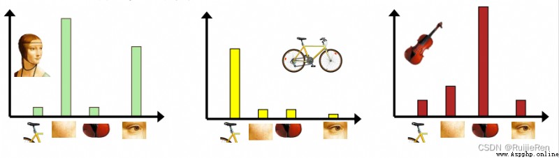
(3) The picture histogram represents
The words in the visual dictionary are used to represent the images to be classified . Calculate... In each image SIFT Feature here K The distance between two visual words ,
among The nearest visual word is this SIFT Visual words corresponding to features .
By counting the number of times each word appears in the image , Represent the image as a K One dimensional numerical vector ,
As shown in the figure , among K=4, Each image is described by histogram :
(4) quantitative
This step is based on image feature extraction , Then the extracted feature points , According to step 3 , Convert to frequency histogram .
Here, when converting to frequency histogram , Have used to TF-IDF, That is word frequency (Term Frequency,TF) And inverse document frequency (Inverse Document Frequency,IDF) The product of As weights . The purpose of introducing this weight is to reduce the impact of some repeated features . For example BOW in , Some common words such as the,it,do And so on , Can not reflect the content characteristics of the text , But the frequency is very high , utilize tf-idf It can reduce the influence of unnecessary words . Empathy , stay BOF Image searching , There will also be such meaningless features between images , Therefore, it is necessary to reduce the weight of such features .
(5) Construct an inverted table
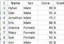
Inverted table is a reverse lookup method , stay BOW The general idea in this article is to use the extracted words , Reverse search for articles with this word . Pictured , Find multiple words , An inverted table is formed .
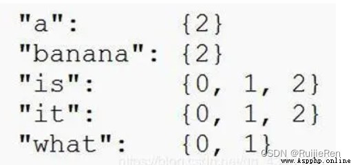
BOF The same is true for the middle inverted table . Through the reverse search of visual vocabulary , You will get a collection of images with the same visual vocabulary , You can get an inverted list by repeating it many times . The inverted table can quickly get new images and similar images in the database .
(6) Match histogram
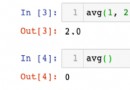
When we finish the above steps , You need to match the histogram . Histogram matching gives the frequency histogram of the input image , Look up... In the database K The nearest neighbor image , According to this K Nearest neighbors vote on the classification results of the image .
TF-IDF(Term frequency-Inverse document frequency) It's a statistical method , Used to evaluate the importance of feature words . according to TF-IDF The formula , The weight of feature words is the same as that in The frequency of occurrence in the corpus is related to , It is also related to the frequency of occurrence in the document . Conventional TF-IDF The formula is as follows :
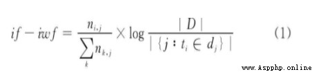
TF-IDF To evaluate the importance of a word to a document set or one of the documents in a corpus . The importance of a word increases in proportion to the number of times it appears in the document , But at the same time, it will decrease inversely with the frequency of its occurrence in the corpus . For now , If one Keywords only appear in very few web pages , Through it, we can Easy to lock the search target , its The weight It should be Big . On the contrary, if A word appears in a large number of web pages , We see it still I'm not sure what I'm looking for , So it's The weight should Small .
TF-IDF The formula is introduced in detail :CSDN Programming community (smartapps.cn)
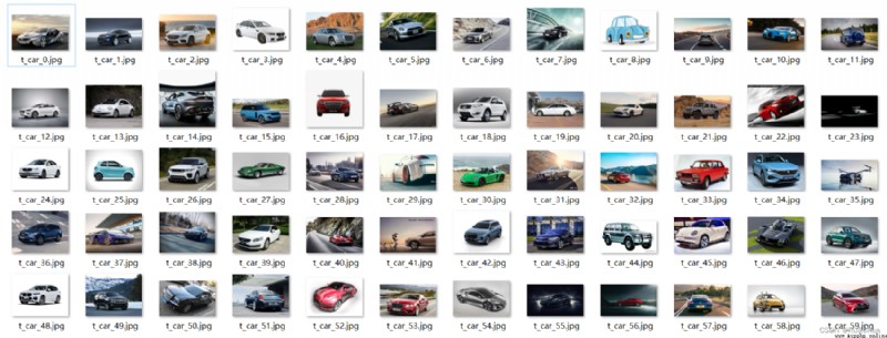
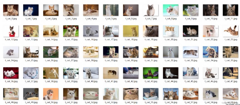
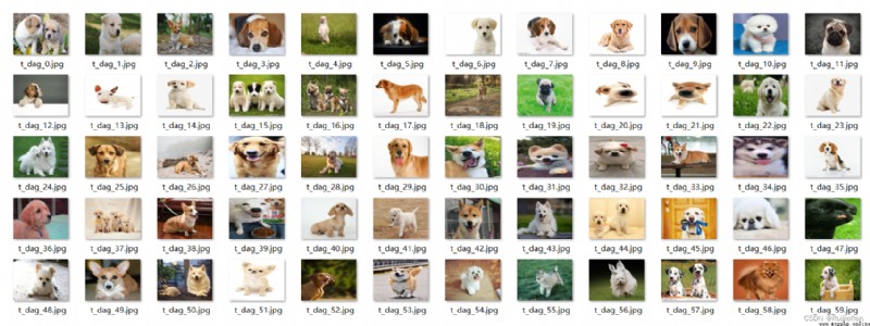
Crawl through the crawler in Baidu to get three kinds of pictures 60 Zhang , And use the batch processing tool to cut all data images to the same size , Uniformly cut to 640*480
A scene :60 A picture of a car
B scene :60 An image of a cat
C scene :60 A picture of a dog
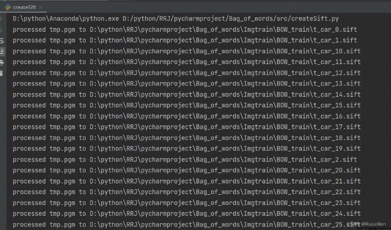
createSift.py
# -*- coding: utf-8 -*-
"""
@author: RRJ
@software: PyCharm
@file: createSift.py
@time: 2022/6/12 22:44
"""
import pickle
from newPCV.imagesearch import vocabulary
from newPCV.tools.imtools import get_imlist
from newPCV.Localdescriptors import sift
# Get image list
imlist = get_imlist('D:\\python\\RRJ\\pycharmproject\\Bag_of_words\\Imgtrain\\BOW_train\\')
nbr_images = len(imlist)
# Get feature list
featlist = [imlist[i][:-3] + 'sift' for i in range(nbr_images)]
# Extract the image under the folder sift features
for i in range(nbr_images):
sift.process_image(imlist[i], featlist[i])
# Generating words
voc = vocabulary.Vocabulary('training')
voc.train(featlist, 180, 10)
# Save vocabulary
# saving vocabulary
with open('D:\\python\\RRJ\\pycharmproject\\Bag_of_words\\BOW\\vocabulary.pkl', 'wb') as f:
pickle.dump(voc, f)
print('vocabulary is:', voc.name, voc.nbr_words)
Training functions :train
def train(self,featurefiles,k=100,subsampling=10):
""" Contain k A word of K-means List in featurefiles A word is trained from the feature file in . Down sampling the training data can speed up the training speed """
nbr_images = len(featurefiles)
# Read features from file
descr = []
descr.append(sift.read_features_from_file(featurefiles[0])[1])
# Put all the features together , For later K-means clustering
descriptors = descr[0]
for i in arange(1,nbr_images):
descr.append(sift.read_features_from_file(featurefiles[i])[1])
descriptors = vstack((descriptors,descr[i]))
#K-means: The last parameter determines the number of runs
self.voc,distortion = kmeans(descriptors[::subsampling,:],k,1)
self.nbr_words = self.voc.shape[0]
# Traverse all training images , And projected onto words
imwords = zeros((nbr_images,self.nbr_words))
for i in range( nbr_images ):
imwords[i] = self.project(descr[i])
nbr_occurences = sum( (imwords > 0)*1 ,axis=0)
self.idf = log( (1.0*nbr_images) / (1.0*nbr_occurences+1) )
self.trainingdata = featurefiles
def project(self,descriptors):
""" Project descriptors onto words , To create a word histogram """
# Image word histogram
imhist = zeros((self.nbr_words))
words,distance = vq(descriptors,self.voc)
for w in words:
imhist[w] += 1
return imhist
Part of the result :
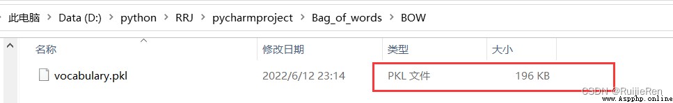
At the same time, the data model is generated vocabulary.pkl, If the data model is empty , An error will be reported when saving in the database later , The read data is empty . Judge .pkl Whether it is empty can be checked according to its size , As shown in the figure below , here pkl by 196KB, Therefore, it is not empty .
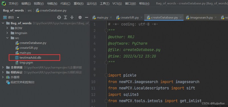
Store the data model obtained above in the database testImaAdd.db in , That is, running the following code will generate a testImaAdd.db Database files .
createDatabase.py
# -*- coding: utf-8 -*-
"""
@author: RRJ
@software: PyCharm
@file: createDatabase.py
@time: 2022/6/12 23:20
"""
import pickle
from newPCV.imagesearch import imagesearch
from newPCV.Localdescriptors import sift
import sqlite3
from newPCV.tools.imtools import get_imlist
# Get image list
# imlist = get_imlist('E:/Python37_course/test7/first1000/')
imlist = get_imlist('D:\\python\\RRJ\\pycharmproject\\Bag_of_words\\Imgtrain\\BOW_train\\')
nbr_images = len(imlist)
# Get feature list
featlist = [imlist[i][:-3] + 'sift' for i in range(nbr_images)]
# load vocabulary
# Load vocabulary
with open('../BOW/vocabulary.pkl', 'rb') as f:
voc = pickle.load(f)
# Create index
indx = imagesearch.Indexer('testImaAdd.db', voc)
indx.create_tables()
# go through all images, project features on vocabulary and insert
# Traverse all images , And project their features onto words ( Let's say mine is 180 A picture )
for i in range(nbr_images)[:179]:
locs, descr = sift.read_features_from_file(featlist[i])
indx.add_to_index(imlist[i], descr)
# commit to database
# Commit to database
indx.db_commit()
con = sqlite3.connect('testImaAdd.db')
print(con.execute('select count (filename) from imlist').fetchone())
print(con.execute('select * from imlist').fetchone())
Running results :
Obtain candidate images using the index + Query with an image + Determine the comparison benchmark and draw the results
Index the image , You can search for similar images in the database . here , Use BOW( The word bag model ) To represent the whole image , It's universal , It can be used to find similar objects 、 Similar faces 、 Similar colors, etc , It all depends on the image and the descriptor used . In order to realize search , stay Imagesearch.py There is Searcher class :
Searcher class :
class Searcher(object):
def __init__(self,db,voc):
""" Initialize with the name of the database. """
self.con = sqlite3.connect(db)
self.voc = voc
def __del__(self):
self.con.close()
def get_imhistogram(self,imname):
""" Return the word histogram for an image. """
im_id = self.con.execute(
"select rowid from imlist where filename='%s'" % imname).fetchone()
s = self.con.execute(
"select histogram from imhistograms where rowid='%d'" % im_id).fetchone()
# use pickle to decode NumPy arrays from string
return pickle.loads(s[0])
def candidates_from_word(self,imword):
""" Get list of images containing imword. """
im_ids = self.con.execute(
"select distinct imid from imwords where wordid=%d" % imword).fetchall()
return [i[0] for i in im_ids]
def candidates_from_histogram(self,imwords):
""" Get list of images with similar words. """
# get the word ids
words = imwords.nonzero()[0]
# find candidates
candidates = []
for word in words:
c = self.candidates_from_word(word)
candidates+=c
# take all unique words and reverse sort on occurrence
tmp = [(w,candidates.count(w)) for w in set(candidates)]
tmp.sort(key=cmp_to_key(lambda x,y:operator.gt(x[1],y[1])))
tmp.reverse()
# return sorted list, best matches first
return [w[0] for w in tmp]
def query(self,imname):
""" Find a list of matching images for imname. """
h = self.get_imhistogram(imname)
candidates = self.candidates_from_histogram(h)
matchscores = []
for imid in candidates:
# get the name
cand_name = self.con.execute(
"select filename from imlist where rowid=%d" % imid).fetchone()
cand_h = self.get_imhistogram(cand_name)
cand_dist = sqrt( sum( self.voc.idf*(h-cand_h)**2 ) )
matchscores.append( (cand_dist,imid) )
# return a sorted list of distances and database ids
matchscores.sort()
return matchscores
def get_filename(self,imid):
""" Return the filename for an image id. """
s = self.con.execute(
"select filename from imlist where rowid='%d'" % imid).fetchone()
return s[0]
def tf_idf_dist(voc,v1,v2):
v1 /= sum(v1)
v2 /= sum(v2)
return sqrt( sum( voc.idf*(v1-v2)**2 ) )
def compute_ukbench_score(src,imlist):
""" Returns the average number of correct
images on the top four results of queries. """
nbr_images = len(imlist)
pos = zeros((nbr_images,4))
# get first four results for each image
for i in range(nbr_images):
pos[i] = [w[1]-1 for w in src.query(imlist[i])[:4]]
# compute score and return average
score = array([ (pos[i]//4)==(i//4) for i in range(nbr_images)])*1.0
return sum(score) / (nbr_images)
Sort the results using geometric properties
This is a common BOW Models are common ways to improve search results .BOW A major of the model The disadvantage is that when using visual words to represent images It does not contain the position information of image features , This is for The cost of getting speed and scalability cost . The most common method is to fit homography between the feature positions of the query image and the front image .
# -*- coding: utf-8 -*-
"""
@author: RRJ
@software: PyCharm
@file: searchImg.py
@time: 2022/6/13 0:43
"""
import pickle
from newPCV.Localdescriptors import sift
from newPCV.imagesearch import imagesearch
from newPCV.geometry import homography
from newPCV.tools.imtools import get_imlist
# load image list and vocabulary
# Load image list
imlist = get_imlist('D:\\python\\RRJ\\pycharmproject\\Bag_of_words\\Imgtrain\\BOW_train\\') # The path where the dataset is stored
nbr_images = len(imlist)
# Load feature list
featlist = [imlist[i][:-3] + 'sift' for i in range(nbr_images)]
# Load vocabulary
with open('../BOW/vocabulary.pkl', 'rb') as f: # Storage path of the model
voc = pickle.load(f)
src = imagesearch.Searcher('testImaAdd.db', voc)
# index of query image and number of results to return
# Query the image index and the number of images returned by the query
q_ind = 18
nbr_results = 5
# regular query
# Regular query ( Sort the results by Euclidean distance )
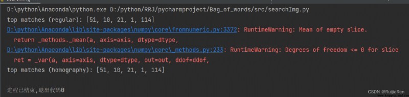
res_reg = [w[1] for w in src.query(imlist[q_ind])[:nbr_results]]
print('top matches (regular):', res_reg)
# load image features for query image
# Load query image features
q_locs, q_descr = sift.read_features_from_file(featlist[q_ind])
fp = homography.make_homog(q_locs[:, :2].T)
# RANSAC model for homography fitting
# Fitting with homography to establish RANSAC Model
model = homography.RansacModel()
rank = {}
# load image features for result
# Load features of candidate images
for ndx in res_reg[1:]:
locs, descr = sift.read_features_from_file(featlist[ndx]) # because 'ndx' is a rowid of the DB that starts at 1
# get matches
# Get the number of matches # get matches After execution, two pictures will appear
matches = sift.match(q_descr, descr)
ind = matches.nonzero()[0]
ind2 = matches[ind]
tp = homography.make_homog(locs[:, :2].T)
# compute homography, count inliers. if not enough matches return empty list
# Calculate the homography , Internal point technology . If there are not enough matching books, an empty list is returned
try:
H, inliers = homography.H_from_ransac(fp[:, ind], tp[:, ind2], model, match_theshold=4)
except:
inliers = []
# store inlier count
rank[ndx] = len(inliers)
# Sort dictionaries , To get the inner points of the innermost layer first
sorted_rank = sorted(rank.items(), key=lambda t: t[1], reverse=True)
res_geom = [res_reg[0]] + [s[0] for s in sorted_rank]
print('top matches (homography):', res_geom)
# Show query results
imagesearch.plot_results(src, res_reg[:8]) # Regular query
imagesearch.plot_results(src, res_geom[:8]) # The result of the rearrangement
The query index is 18 Image , Running results :

The query image is on the far left , The following are the front images retrieved according to the image list 5 Images .
On the output of the results , First of all Load image list 、 Feature list and vocabulary . then Create a Searcher object , Perform periodic queries , And save the results in res_reg In the list , Then load res_reg Each image feature in the list , And match with the queried image . By calculating the number of matches and counting the number of points inside, we get , Finally, the dictionary containing image index and interior points can be sorted by reducing the number of interior points . Finally, visually retrieve the matching image results in the front .
The query index is 100 Image , Running results :

 It can be seen that the wrong image appears in the search here , And it is obviously found that the two types of images are significantly different , Guess the wrong reason is that the data set is too small or K Too big a reason .
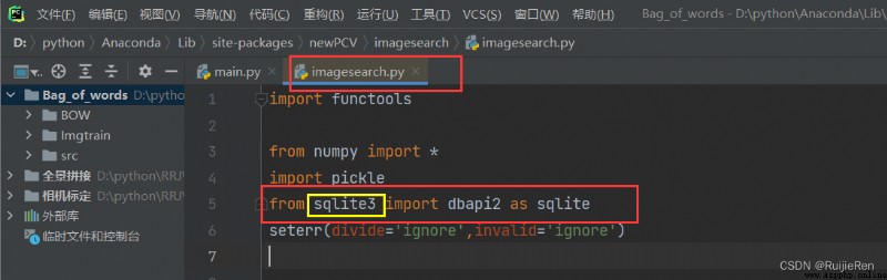
(1)ModuleNotFoundError: No module named 'pysqlite2'
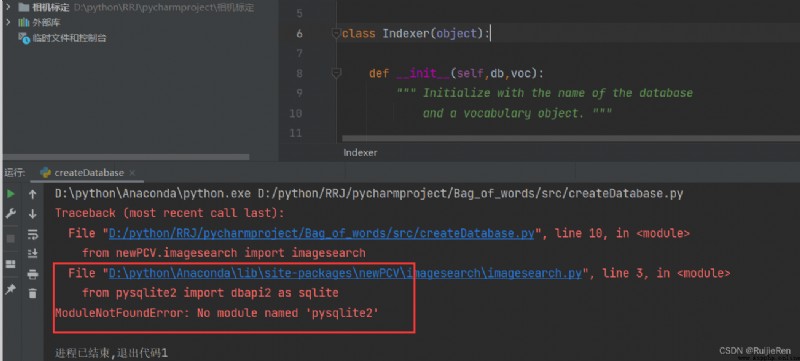
resolvent : Check online ,python3 No longer supported pysqlite2 This is the library , Find yourself imagesearch.py The path where the file is located , Modify the red line area as shown in the figure , And ensure your python Has been successfully installed pysqlite3 package .
(2)TypeError: 'cmp' is an invalid keyword argument for sort()
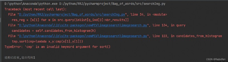
resolvent : Find the target file and modify it according to the following figure 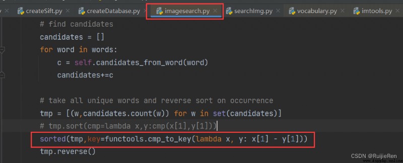
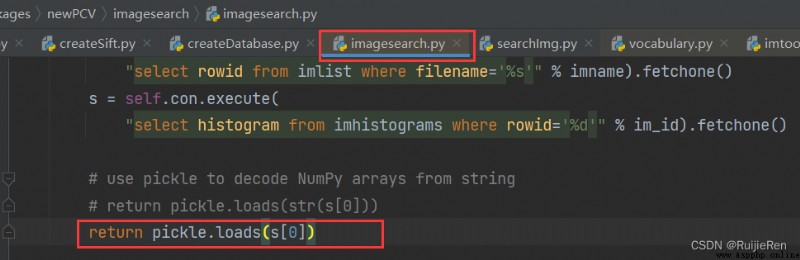
(3)TypeError: a bytes-like object is required, not 'str'
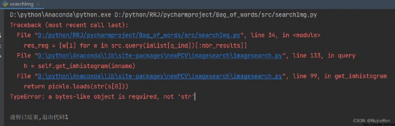
resolvent :
(1) Computer vision —— Image retrieval and recognition _Nikki_du The blog of -CSDN Blog _ Image recognition and image retrieval
(2)python Computer vision - Image retrieval and recognition _ I love it Debug The blog of -CSDN Blog _python Visual recognition