Resource download address :https://download.csdn.net/download/sheziqiong/85705488
Resource download address :https://download.csdn.net/download/sheziqiong/85705488
" Pat loans " The data provided includes the credit default tag ( The dependent variable )、 Basic and machining fields required for modeling ( The independent variables )、 Raw data of network behavior of relevant users , The data field has been desensitized . The actual combat is based on the preliminary data , Include 3 Ten thousand training sets and 2 Ten thousand test sets . Data documents include :
Master: Each line represents a sample ( A successful transaction loan ), Each sample contains 200 Multiple types of fields .
Log_Info: The borrower's login information , Each sample contains multiple pieces of data .
Userupdate_Info: The borrower modifies the information , Multiple pieces of data per sample .
Build prediction model based on training set data , Use the model to calculate the score of the test set ( The higher the score , The more likely it is to default on the loan ), The evaluation criteria are AUC.
Data cleaning work , It mainly deals with missing values , Constant variable processing , Space character processing , Character case conversion, etc
Feature processing work , It is divided into feature transformation and feature derivation . Mainly did the following work :
Master data : Processing of geographic location information ( Province , City ), Transformation of operators and microblog features , And sorting characteristics ,periods Cross combination of features, etc .
Log_Info data : Derived from " Cumulative login times ",“ The average interval between logins ”," The difference between the last login time and the transaction time " Other characteristics .
Userupdate_Info data : Derived from " Difference between the latest modification time and the closing time ",“ The total number of times the information was modified ”, " The number of times each message is modified " Other characteristics .
Feature screening : utilize lightgbm Output feature importance for filtering .
Modeling work :
Single model , The selected machine learning model is lightgbm.
bagging Model : be based on bagging Thought , Through random disturbance of model parameters , Build multiple sub models , The selected base model is lightgbm.
Data outlier determination , cleaning
utilize XGboost, Derive new features according to the feature importance system , Peel off useless features
Discretization of features , Two valued , Numerical feature derivation sort
Cross validation , Grid search complete lightGBM Super parameter settings
bagging lightGBM Model
Mater The data contains about 50000 Samples ,200 Multiple fields .
# The quality ratio of the sample
data1.target.value_counts()

It's better than worse 11:1, Belongs to an unbalanced dataset , Because the final model uses lightgbm, Therefore, oversampling method will not be used for data sampling in this practice , Modeling directly from raw data .
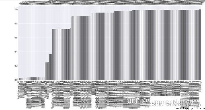
Data visualization of missing variables

There are some variables with high missing rates , If the missing is filled with 0, This kind of variable can be regarded as a kind of sparse feature , because xgboost,lightgbm etc. GBDT The class tree model is not very good at processing high-dimensional sparse features , And considering that the business meaning of these variables is unknown , Carrying too little information , Therefore, the variables with high missing rate are deleted .
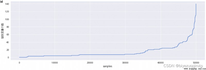
In addition to considering the absence of variables , The number of missing features of the sample should also be considered , If a sample has many missing features , It means that the information of users is not perfect , Through the visualization of missing samples , These outliers are found , Consider deleting .
# Visualization of trend number of samples
sc.plot_missing_user(df=data1,plt_size=(16,5))

# The number of missing deleted variables is 100 More than users
data1 = sc.missing_delete_user(df=data1,threshold=100)
The number of missing variables is 100 The number of users above is 298 individual .
When the proportion of a single value in a variable is too high (90% above ), It shows that the variance of this variable is relatively small , Carry less information , Resulting in poor discrimination , These variables are also deleted .
Urban feature cleaning :
# Calculation 4 Non repeating item count of city features , Observe whether there is any abnormal data
for col in ['UserInfo_2','UserInfo_4','UserInfo_8','UserInfo_20']:
print('{}:{}'.format(col,data1[col].nunique()))
print('\t')

UserInfo_8 Relative to other features nunique more , I found that some cities have " City ", Some don't , You need to do some format conversion , Remove the string suffix " City ".
print(data1.UserInfo_8.unique()[:50])

# UserInfo_8 Cleaning treatment , After processing, the non duplicate count decreases to 400
data1['UserInfo_8']=[s[:-1] if s.find(' City ')>0 else s[:] for s in data1.UserInfo_8]
UserupdateInfo1 Feature case conversion :
'UserupdateInfo1’ Contains case , Such as "qQ" and "QQ", Belong to the same meaning , Therefore, it is necessary to convert English characters to upper and lower case .
# take UserupdateInfo1 Change the characters in to lowercase
df2['UserupdateInfo1'] = df2.UserupdateInfo1.map(lambda x:x.lower())
Yes Master Category type features in ( Province , City , Operator, , Microblogging ) Do feature conversion , Sort numeric variables ,periods Derivation of features .
Category features :
The original data has two province fields , Guess a registered residence address of the user , The other is the province where the user lives , The fields that can be derived from this are :
Province binarization , A single province is derived into a binary feature through the default rate , It is divided into registered residence province and residence province
Whether the province of registered residence and the province of residence are consistent , It is speculated that most of the inconsistent users are migrant workers , The relative default rate will be a little higher .
The number of borrowers in the province should be taken into account when calculating the default rate , If the number is too small , Reference value is not great
Province binarization

The top five provinces with the highest default rate are selected from the two provincial characteristics , And do binary derivation .
The difference between the province of registered residence and the province of residence
In the original data are 4 City Information , It is speculated that the user often logs in IP Address city , The derived logic is :
adopt xgboost Select the more important urban variables , Carry out binary derivation
from 4 The non repeated item count of urban features can be derived Sign in IP Number of address changes
Urban dualization is derived
# according to xgboost The output of variable importance makes binary derivation to the city

The top three cities in terms of feature importance will be derived from the binary system :
IP Address change times derivation
Because there are few types of operators , Just do subcoding directly .
First, fill in the missing values for the microblog features , Then do subcoding .
Numerical features :
Sort numeric features from small to large , Derived into sorting features , The sorting feature outliers have stronger robustness , It can enhance the stability of the model , Reduce risk of over fitting .
# Build contains only periods A temporary watch
periods_col = [i for i in num_col2 if i.find('Period')>0]
periods_col2 = periods_col+['target']
periods_data = data1.loc[:,periods_col2]
Observation contains period1 Data for all fields , It is found that the magnitude difference between fields is large , May mean different things , Not suitable for derivatives .
periods1_col = [col for col in periods_col if col.find('Period1')>0]
periods_data.loc[:,periods1_col].head()

Observe that the suffixes are 1 Field of , It is found that the magnitude of field data is basically the same , You can do min,max,avg The derivation of such statistical values .
period_1_col=[]
for i in range(0,102,17):
col = periods_col[i]
period_1_col.append(col)
periods_data.loc[:,period_1_col].head()

All suffixes are 1 Of periods Fields do the corresponding four operations ( Minimum , Maximum , Average ), Derived into new features .
Derived variables
Cumulative login times
The average interval between logins
The difference between the last login time and the transaction time
Derived variables
Summarize derived features into a table :
update_info = pd.merge(time_span,cate_change_df,on='Idx',how='left')
update_info = pd.merge(update_info,update_cnt,on='Idx',how='left')
update_info.head()
1. Single model lightgbm(single_lightgbm_model Code module )
sklearn Interface version
[ Failed to transfer the external chain picture , The origin station may have anti-theft chain mechanism , It is suggested to save the pictures and upload them directly (img-PwC1RKaq-1655693041517)(https://www.writebug.com/myres/static/uploads/2022/6/18/b8b514598c8d1312831c6c39cc33ea46.writebug)]
The original version of lightgbm

Adjustable parameter
# Determine the maximum number of iterations , The learning rate is set as 0.1
base_parmas={'boosting_type':'gbdt',
'learning_rate':0.1,
'num_leaves':40,
'max_depth':-1,
'bagging_fraction':0.8,
'feature_fraction':0.8,
'lambda_l1':0,
'lambda_l2':0,
'min_data_in_leaf':20,
'min_sum_hessian_inleaf':0.001,
'metric':'auc'}
cv_result = lgb.cv(train_set=lgb_train,
num_boost_round=200,
early_stopping_rounds=5,
nfold=5,
stratified=True,
shuffle=True,
params=base_parmas,
metrics='auc',
seed=0)
print(' Maximum number of iterations : {}'.format(len(cv_result['auc-mean'])))
print(' Cross validated AUC: {}'.format(max(cv_result['auc-mean'])))
determine subsample by 0.5,colsample_bytree by 0.6
[ Failed to transfer the external chain picture , The origin station may have anti-theft chain mechanism , It is suggested to save the pictures and upload them directly (img-6K6spI9z-1655693041520)(https://www.writebug.com/myres/static/uploads/2022/6/18/981a2f24600efae4e882a964a55f7894.writebug)]
determine reg_lambda by 0.03,reg_alpha by 0.3

Determine the final number of iterations as 889 Time
lgb_single_model = lgb.LGBMClassifier(n_estimators=900,
learning_rate=0.005,
min_child_weight=0.001,
min_child_samples = 20,
subsample=0.5,
colsample_bytree=0.6,
num_leaves=30,
max_depth=-1,
reg_lambda=0.03,
reg_alpha=0.3,
random_state=0)
lgb_single_model.fit(x_train,y_train)
pre = lgb_single_model.predict_proba(x_test)[:,1]
print('lightgbm Single model AUC:{}'.format(metrics.roc_auc_score(y_test,pre)))
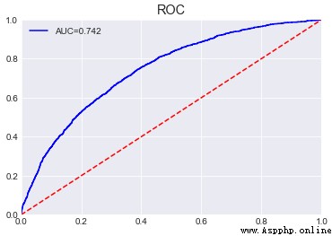
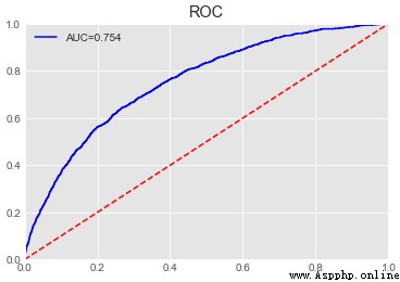
sc.plot_roc(y_test,pre)

Test set after parameter adjustment AUC Promoted 0.015.
It mainly draws lessons from the idea of the randomness of random forest for selecting samples and the randomness of characteristics .
Implementation method of sample randomness :random_seed,bagging_fraction,feature_fraction Parameter perturbation of
Implementation method of characteristic randomness : Based on the use of all native features , Random extraction of certain sorting features and periods Feature into model .
Resource download address :https://download.csdn.net/download/sheziqiong/85705488
Resource download address :https://download.csdn.net/download/sheziqiong/85705488